Modeling a Three-Pendulum Harmonograph – tutorial: part #2

Hi guys, here is the second part of a tutorial describing the matematical equations used in modeling a three-pendulum harmonograph (automatic drawing machine). It pertains to the second version of the model.

This section describes the kinematic equations involved in the articulated linkage mechanism on the top of the table, the custom spreadsheet functions used in the model and some overall considerations about the partition of the spreadsheet.  This is an advanced tutorial so you need a minimum of high-school physics and geometry background. So what do you think?

Cheers,
George

[sociallocker][/sociallocker]

Modeling a Three-Pendulum Harmonograph – Part #2 – by George Lungu

 

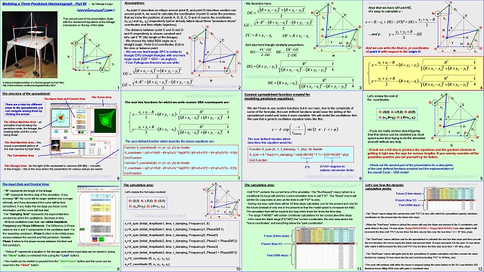
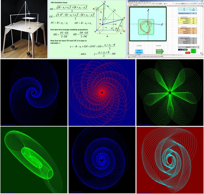
This second part of the presentation deals with the movement equations of the linkage mechanism on the top of the table.

(Writing table)

A physical implementation of a harmonograph by Karl Sims

<excelunusual.com> 1

 

Assumptions:

– As point C describes an ellipse around point B, and point D describes another one around point A, we need to calculate the coordinates of
point G under the premises that we know the positions of points A, O, B, C, D and of course the coordinates (x1,y1) and (x2, y2) respectively
(we’ve already talked about these “pendulum-driven” coordinates and their elliptic trajectory).

-The distance between point C and G and D and G respectively is chosen constant and 2 let’s call it “R” (the length of the linkage).

– We choose the initial BOA angle as a straight angle. Point O of coordinates (0,0) is the zero or balance point.

– We can see that triangle DFC is similar to triangle EHG (straight triangles with one more angle equal (CDF = GEH – as angles))

– From Pythagoras theorem we can write:
–

We therefore have:

And also from triangle similarity proportions:

Now that we have GH and HE, it’s easy to calculate x :

And we can write the final (x, y) coordinates of point G with respect to the origin O:

<excelunusual.com> 4

Let’s review the rest of  the coordinates:

O: (0,0) A: (-R,0) B: (0,R)
C: (x2,R+y2) D: (-R+x1, y1) F

– If you are really serious about figuring how this device can be modeled you must spend some time trying to do the derivation
yourself without any help.

– It took me a full day to produce the equations and the greatest obstacle in getting it right was the sign for various lengths. If you naively consider all the
quantities positive you set yourself up for failure.

– Check out the second part of the presentation for a description of the user defined functions involved and the implementation of the overall Excel – VBA model

<excelunusual.com> 5

 

Custom spreadsheet function created for modeling pendulum equations:

We don’t have to use custom functions but in our case, due to the complexity of some of the formulas, the user defined functions would ease the writing of the
spreadsheet model and make it more readable. We will model the oscillations first. We saw that a generic oscillation equation looks like this:

The user defined function which describes this equation would be:

Function X_spin (A, t, t_damping, f, phy) As Double
X_spin = A * Exp(-t / t_damping) * sin(6.283185 * f * t + 0.01745329 * phy)
End Function

pi/180= degrees to radians conversion factor

<excelunusual.com> 6

The next two functions for which we write custom VBA counterparts are:

The user defined function which describe the above equations are:

Function X_coordinate(R, x1, y1, x2, y2) As Double
X_coordinate = (x2+x1-R)/2 + (R+y2-y1) * Sqr(R^2 / ((R+x2-x1)^2 + (R+y2-y1)^2) – 0.25)
End Function

Function Y_coordinate(R, x1, y1, x2, y2) As Double
Y_coordinate = (y2+y1+R)/2 – (R+x2-x1) * Sqr(R^2 / ((R+x2-x1)^2 + (R+y2-y1)^2) – 0.25)
End Function

<excelunusual.com> 7

 

The structure of the spreadsheet:

The Curve Area
The Input Data and Control Area

There are a total six different areas in the spreadsheet, you can navigate among them by clicking the arrows:
The Virtual Machine Area – an animated chart showing the pendulum ends, the linkage, the drawing table and the curve being drawn.
The Real Machine Area – this is just a annotated picture of the real machine by Karl Sims
The Calculation Area
The Storage Area – (to the right of the worksheet in columns (BA:BB) – not seen in this image) – this is the area where the parameters
for various setups are saved

<excelunusual.com> 8

 

The Input Data and Control Area:

– “R” represents the length of the linkage

– “dt” represents the time step of the simulation. If you increase “dt” the curve will be larger (plotted over a longer interval), and if you decrease
it the curve will be finer (smoother). If you make this too large you loose curve information and the curve will look bad.

-The “Damping Time” represents the exponential time constant by which the oscillations decrease in time.

– All three oscillators have their own Initial Amplitude, Frequency and Phase Difference.

 

The Difference in Phase refers to the X and Y components of the oscillation itself.

For the respective pendulum, Phase 2 refers to the initial phase excess between the second and first pendulum. Similarly

Phase 3 refers to the phase excess between the third and first pendulum.

– “Setup #” represents a location in the storage area where input data can be stored in (using the “Store” button) or retrieved from (using the “Load” button).

– The model can be started or paused from the “Start-Pause” button and the curve can be reset from the “Reset” button:

<excelunusual.com> 9

 

The calculation area:

Let’s review the formulas involved:

O: (0,0) A: (-R,0) B: (0,R) F

C: (x2,R+y2) D: (-R+x1, y1)

1
x1=X_spin (Initial_Amplitude1, time, t_damping, Frequency1, 0)
y1=X_spin (Initial_Amplitude1, time, t_damping, Frequency1, PhaseDiff.1)
x2=X_spin (Initial_Amplitude2, time, t_damping, Frequency2, Phase2)
x2=X_spin (Initial_Amplitude2, time, t_damping, Frequency2, Phase2 + PhaseDiff.2)
x3=X_spin (Initial_Amplitude3, time, t_damping, Frequency3, Phase3)
x3=X_spin (Initial_Amplitude3, time, t_damping, Frequency3, Phase3 + PhaseDiff.3)
xG=X_coordinate (R, x1, y1, x2, y2)
xG=Y_coordinate (R, x1, y1, x2, y2)

<excelunusual.com> 10

 

The calculation area:

-Cell “F57” contains the current time of the simulation. The “RunPause()” macro (which is a conditional Do loop) will print the current
simulation time in cell “F57”. The “Reset” macro will set the Do Loop index to zero an the time in cell “F57” to zero.

– During one loop cycle there will be 10 time steps calculated, one for the present and nine for the future (instead of only one in the present so
that the model speed is increased ten fold). The simulation time will be equal to the loop index times ten times the time step.

– The range “F48:N57” will contain coordinate calculations for ten consecutive time steps

– Let’s name the black range (F57:N57) the “current coordinates, the nine rows above the “future coordinates” and everything below the “past coordinates”.

Future (9 time steps)
Present (Row 57)
Past (5000 steps)

<excelunusual.com> 11

 

Let’s see how the dynamic calculation works:

Future (9 time steps)
Present (Row 57)
Past (5000 steps)

– The “Reset” macro brings the current time (cell “F57”) to zero after which he spreadsheet quickly calculates coordinates for the present plus
the future nine steps.

– When the “RunPause” button is clicked the macro will copy the future and present of the G coordinates and paste them in the past, 10 rows down:
Range(“M58:N5058”) = Range(“M48:N5048”).Value after which it will increment the time (cell “F57”) by ten times the time step (in this case the
new time = 0 + 10* time_step).

– The “RunPause” macro will then wait for the spreadsheet to calculate the next ten time steps and then execute the next iteration: the macro copies
the future and present (total 10 rows) and paste it in the past 10 rows down after which it will increment the time (cell “F57”) by ten times the time step
(new time = 20* time_step).

– The “RunPause” macro will again wait for the spreadsheet to update calculation and then execute the same iteration by copying 10 rows down into the
past and incrementing “F57” to 30*time_step.

-The cycle will continue until either the macro is stopped (using the same button) or the Do Loop finishes 500 iterations hence filling 5000 rows with
point G coordinate data.

by George Lungu <excelunusual.com>