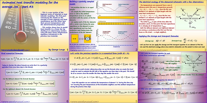
This section shows how to model heat transfer in a linear bar by dividing it in elementary sections in which the basic linear equations introduced in the previous tutorials can be used.
![]()
Animated heat transfer modeling for the average Joe – part #3
by George Lungu
– This is a new section of the
beginner series of tutorials in heat
transfer modeling. The first part
introduced the reader to the
concept of heat capacity and heat
conductance and the linear laws
that connect temperature with
the aforementioned properties.
– This section shows how to model
heat transfer in a linear bar by
dividing it in elementary sections
using the basic linear temperature
equations introduced in the
previous two tutorials.
by George Lungu
<excelunusual.com>
Building a spatially sampled model: Initial temperature Ambient temperature curve curve
– We partition the bar in 21 equal
samples.
– We sample the initial temperature x
curve as well as the ambient temperature curve in 21 places
coincident with the centers of the bar elements.
– We replace each of the bar elements
with a center mass having the same
capacitance as the element (a pure
heat capacitance) and two heat
conductors each having twice the
Sampled initial
Sampled ambient
conductance of the bar element:
temperature temperature
C / G C, x
We use twice the conductance because when we
connect the elements in series we get a 1G resultant
conductance between consecutive element centers.
<excelunusual.com> 2
The electrical analogy of the elemental schematic with a few observations:
– The temperatures are measured from a zero K
reference point (the zero K temperature ground).
– G1 = G2 = … =Gn = … = G21 since the bar was
divided in 21 elements of equal length with the
same heat conductance.
– C1 = C2 = … =Cn = … = C21 since the bar was
divided in 21 elements of equal length with the Tn 1
same heat capacitance.
– The switch Sinitial is open all the time after the simulation starts. At that point the heat capacitance
Cn is already set at temperature Tinitial_n
– Both the leftmost element and rightmost element
are missing a conductance (the first and the last
house on the street – a single neighbor).
Applying the storage and transport formulas:
dQ
(storage eq.) dQ C dT (transport eq.) G(T T )
1 2
dt
– Let’s see how we can apply the storage and the transport equation to an element of the bar.
– We used the electrical analogy above since electric schematics are the easiest to draw and read.
<excelunusual.com> 3
– Let’s write the transport equation for each of the three conductances separately: initial_n ambient_n
from left neighbor
– rate of heat transfer from the ambient
– Now let’s write the storage equation for element n:
dQ t) dQ t)dQ t)dQ t) CdT (t)
– After some light manipulation the formula becomes:
Gdt T t)T t)2T t)G dt T t) T t) CdT t)
Let’s write the previous equation in a numerical form (with dt = h):
Gdt T t)T t)2T t)G dt T t) T t) CdT t)
Gh T (m)T (m)2T (m)G h T (m)T (m ) C T (m)T (m1)
n1 n1 n ambient ambient_n n n n
– In order to avoid circular referencing when we use the formula when we create the Excel
model we need to evaluate the left side of the equation one time step in the past. This should
be of no concern since the smaller the time step the smaller the error:
Gh T (m1)T (m1)2T (m1)G h T (m1)T (m1 ) C T (m)T (m1)
– From this equation we can evaluate the temperature of element “n” during the time step
“m” knowing the past temperatures of the immediate neighbors and the ambient temperature
during the previous time step:
T (m) T (m1) T (m1)T (m1)2T (m1) T (m1)T (m1 )
<excelunusual.com> 5
Final numerical formulas:
T (m) T (m1) T (m1)T (m1)2T (m1) T (m1)T (m1 )
Trying to shorten the above formula we write the it in a perfectly
equivalent form (one time step in the future):
T (m1) T (m) T (m)T (m)2T (m) T (m)T (m )
For the leftmost element the formula becomes:
T (m1) T (m) T (m)T (m) T (m)T (m )
For the rightmost element the formula becomes:
T (m1) T (m) T (m)T (m) T (m)T (m )
The three formulas above are all we need to model heat transfer in a uniform rod in Excel.
to be continued…
by George Lungu <excelunusual.com> 6


I can’t think of a real world example where materials would have the initial temp curve and ambient temp curve described in this model.It seems to me a temperature profile as a function of distance heat transfered into materials would be a more practical model. Which I guess can be easily done using the same principle. Thx again on behalf of average joes.
Thanks for the comment. They are both equivalent and you can easily change the model to do what you say. Just wait till I post the last part (late this afternoon). No model can cover all situations but take for instance a connection rod or a valve in an engine during operation, or a house during a night-day cycle. They are almost perfect examples of starting initial temperatures by a map (during the night the house settles to some distribution of temp. and during the day you’ve got the sun going around and heating the house and the air at the Eastern side in the morning and Western side in the afternoon. You need minutes to adjust the model for this plus you can introduce radiation, Stefan Bolzman etc. My purpose is not to give the perfect tool but to show the principle of modeling. If you understand it you can easily make any model you like with all the secondary effects and parameters you need. Cheers, George
Another example which fits my model is when you harden a steel object, you insert various parts in various liquids to get different hardness and resilience across the length. Or think about a satelite aimed at with a laser weapon. You need to design the thickness of the wall, conductivity and reflectivity so that the beam heat disperses to the neighboring areas without melting the contact spot. I can go on and on.
If you take the heat transfer profile rather than ambient temp. profile, the formula actually simplifies. Try to create your own. The purpose of the pwebsite is to encourage you to make your own models much different and better (fit to your application) than what you see here.