Animated Heat Transfer Modeling for the Average Joe – part #4

This is the last tutorial of the series and it shows how to implement the previously derived formulas into a spreadsheet model.

The spreadsheet formulas, the macros and charting of the dynamic data is explained.

[sociallocker][/sociallocker]

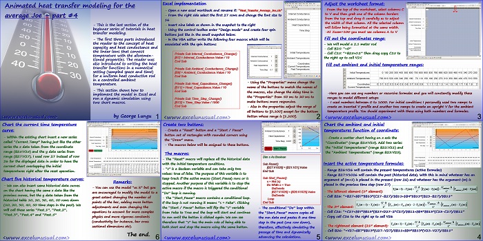
Animated heat transfer modeling for the average Joe – part #4

by George Lungu

– This is the last section of the
beginner series of tutorials in heat
transfer modeling.

– The first three parts introduced
the reader to the concept of heat
capacity and heat conductance and
the linear laws that connect
temperature with the aforemen-
tioned properties.

The reader was
also introduced to writing the heat
transfer functions in a numerical
setting (sampled space and time)
for a uniform heat conductive rod
in a controlled ambient
temperature.

– This section shows how to
implement the model in Excel and
run a dynamic simulation using two short macros.

by George Lungu

<excelunusual.com>

Excel implementation

– Open a new excel workbook and rename it: “Heat_Transfer_Average_Joe.xls”

– From the right side select the first 27 rows and change the font size to 16

– Insert nine labels as shown in the snapshot to the right

– Using the control toolbox enter “Design mode” and create four spin
buttons just like in the small snapshot below.

– In the VBA editor write the following four macros which will be
associated with the spin buttons:

Private Sub Internal_Conductance_Change()
[B7] = Internal_Conductance.Value / 10
End Sub

Private Sub Ambient_Conductance_Change()
[B9] = Ambient_Conductance.Value / 10
End Sub

– Using the “Properties” menu change the name of the buttons to match the names of the macros, also change the delay time in
the “Properties” from 50 ms to 20 ms to make buttons more responsive.

Private Sub Heat_Capacitance_Change()
[B11] = Heat_Capacitance.Value / 10
End Sub

Private Sub Time_Step_Change()
[B13] = Time_Step.Value / 1000
End Sub

– Also in the properties adjust the range of all buttons to [0,100] except for the bottom button whose range is [1,100].

<excelunusual.com> 2

Adjust the worksheet format:

-From the top of the worksheet, select columns C
to V and then grab one of the column borders
from the top and drag it carefully as to adjust
the width of that column. All the selected column
will follow being formatted at the same width.

-At Zoom=100 you must see columns A to V

Fill out the coordinates range:

– We will model a 2.1 meter rod
– Cell B25: “=0”
– Cell C25: “=B25+0.1” then drag copy C25 to the right up to cell V25

Fill out ambient and initial temperature ranges:

-Here you can use any numbers or recursive formulas and you will constantly modify these
ranges to model different setups

– I used numbers between 0 to 1000. For initial conditions I personally used two ramps to
create an inverted V profile and another two ramps to create an upright V for the ambient
temperature profile. You should experiment with these using both numbers and formulas.

<excelunusual.com> 3

Chart the ambient and initial temperatures function of coordinate:

– Create a scatter chart having on x axis the
“Coordinates” (range B25:V25). Add two series:
the “Initial Temperatures” (range B21:V21) and
the “Ambient Temperatures” (range B23:V23).
Insert the active temperature formulas:

– Range B26:V26 will contain the present temperatures (active formulas)

– Range B27:V1026 will contain the past (historical data). With this in mind whatever has an
argument of (m+1) is placed in the present (row 26) and whatever has the argument (m) is
placed in the previous time step (row 27)

Gh G h
ambient
T (m1) T (m)   T(m)T (m)   T (m)T (m )
1 1 2 1 ambient_n 1

– The leftmost element (1st element): C C

– Cell B26: “=B27+$B7*$B13*(C27-B27)/$B11+$B9*$B13*(B23-B27)/$B11”
Gh G  h
ambient
T (m 1) T (m)    T (m)T (m)2T (m)   T (m) T (m )
n n n1 n1 n ambient_n n

– The 2nd element: C C
– Cell C26: “=C27+$B7*$B13*(B27+D27-2*C27)/$B11+$B9*$B13*(C23-C27)/$B11”
– Copy cell C26 to the right up to cell V26
Gh G h
ambient
T (m1) T (m)   T (m)T (m)   T (m)T (m )
21 21 20 21 ambient_n 21

– The rightmost element (21st element): C C

– Cell V26: “=V27+$B7*$B13*(U27-V27)/$B11+$B9*$B13*(V23-V27)/$B11”

<excelunusual.com> 4

Create two buttons:

– Create a “Reset” button and a “Start / Pause”
button out of rectangles with rounded corners using
the “Draw” menu.

– The macros below will be assigned to these buttons.

The macros:

Dim s As Boolean
– The “Reset” macro will replace all the historical data
with the initial temperature conditions.

Sub Reset()
[B27:V1026] = [B21:V21].Value
End Sub

– “s” is a Boolean variable and can take only two values: true of false. The purpose of this variable is to keep track if the active macro (Start_Pause) runs or is stopped. Another purpose of this variable is to stop the active macro if the macro is triggered when the DoEvents conditional “Do” loop is running.

Sub Start_Pause()
s = Not (s)
Do While s = True
[B27:V1026] = [B26:V1025].Value

Loop
End Sub

– The “Start_Pause” macro contains a conditional loop.
If the loop is not running it means “s = False”. Clicking
the “Start / Pause” button will flip the “s” variable
from False to True and the loop will start and continue the “Start_Pause” macro copies all
to run until the button is clicked again.

We can see the run data and pastes it one time
therefore that “s” has the main role of being able to step in the past (one row down),
both start and stop the macro using the same button. therefore, effectively simulating the
passage of time and dynamically advancing the calculations.

<excelunusual.com> 5

Chart the current time temperature curve:

– Within the existing chart insert a new series
called “Current_Temp” having just like the other
series the x data taken from the coordinate
range (B25:V25) and the y data series from
range (B27:V27).

I used row 27 instead of row
26 for the displayed data in order to have the
current chart overlapping the initial
temperatures right after the reset operation.

Chart five historical temperature curves:

Remarks:

– We can also insert some historical data curves

– You can use the model “as is” but you
on the chart having the same x data like the
are encouraged to modify the model to a
previous curves, but the y data taken from the
great extent changing the number of
historical table 10, 20, 30, 40, 50 rows down
points of the bar, adding more button
(10, 20, 30, 40, 50 time steps in the past). We
adjustments and even changing the
will call these series “Past_1”, “Past_2”,
equations to account for more complex
“Past_3”, “Past_4” and “Past_5”
physics and more rigorous constants
(conductivity for instance, bar cross
sectional dimensions etc).
The end.

by George Lungu <excelunusual.com> 6