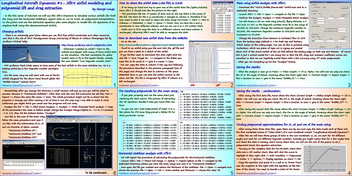
This is a tutorial about using a free aerodynamic modeling package (Xflr5) to simulate two airfoils in 2D (the main wing and the horizontal stabilizer) for ten different Reynolds numbers, then using Excel to extract the approximate polynomial equations of those curves (cl, cd and cm) and based on them, simulate a 2D aircraft as an animated model. This section deals with the aero modeling and the 4th and 5th order polynomial extraction.
Longitudinal Aircraft Dynamics #1- Xflr5 airfoil modeling and polynomial lift and drag extraction
by George Lungu
– In the this series of tutorials we will use the Xflr5 freeware to simulate various airfoils (for both
the wing and the horizontal stabilizer), export resulting data as .csv to Excel, do polynomial
interpolations on the polars and use the extracted equations plus some physics to model the 2D
dynamics of an airplane built using the aforementioned airfoils.
Choosing airfoils:
– There is an extremely good place where you can find free airfoil coordinates and other resources,
and that is the site of UIUC Aerodynamics Group (University of Illinois at Urbana Champaign) led by
professor Michael Selig:
https://www.ae.illinois.edu/m-selig/index.html
– Whenever I needed an airfoil I went to the
website and played with many of those airfoil data
on the simulator. The best candidates for glider
models seem to be in the Eppler family, namely
the ones labeled “Low Reynolds number data”.
– MIT professor Mark Drela seems to have some of the best airfoils in the same database too. He is a leading authority in low Reynolds number aerodynamics.
– For the main wing we will start with one of Mark’s
airfoils designed for the discus hand launch glider the
“Bubble Dancer” named AG24.
<excelunusual.com>
1
How to chart the airfoil data (.dat file) in Excel:
– If we bring up Excel and try to open one of the airfoil data file (Spline_Foil.dat)
from Xflr5 it should look like the picture to the right.
– This particular file has 160 points of data and on the top there is the name of
the foil. The data for the x-y coordinates is merged in column A, therefore if we
ever need to plot it we need to select the data range (A2:A60) => Data => Text
to Columns => Delimited => Next => Space => Finish. Now we have the x and y
coordinates in two different columns and we can use it in a 2D scatter chart.
– Make sure to first copy the data to a different column and leave column A
unchanged, otherwise Xflr5 won’t be able to recognize the .dat airfoil format.
How to download new airfoil data from the website:
– Go to the site:
– Scroll to an airfoil entry you like and click the .gif file and
you can have a peek at a sketch of the airfoil.
-If you decided to download this data right click the
.dat file => Save Target As… => navigate to the folder you
need this to be saved in => give it a name => Save
-You can copy the data in column D lets say, and following
the procedure described in the previous paragraph (top of
this page) change the text to columns in the space
delimited form so you can plot the airfoil contour in the
same .dat file. The file is still recognized by Xflr5 if column
A is left unchanged.
<excelunusual.com>
2
Main wing airfoil analysis with Xflr5:
– Download the “AG24_Bubble_Dancer.dat” airfoil and save in a
dedicated directory.
– Launch Xflr5 => File => Open => navigate to the file => Open
– Perform the analysis: Analysis => Multi-threaded Batch Analysis
– We will choose a 20 cm wide wing (chord), flying between 1.5
m/s and 15 m/s so the Reynolds number must be in the range of
20,000 to 200,000. Change the minimum Reynolds number to
20,000, the maximum Reynolds number to 200,000 and the
increment to 20,000.
– Change the transition from laminar to turbulent flow to 20%
from the leading edge (default is 1 for both top and bottom,
which means at the railing edge). You can do this in practice using
turbulators which are pieces of tape cut in zigzag and pasted
about 20% of the chord (width of the air foil) behind the leading edge on both top and bottom. Of course
this is just a virtual model but I am doing this so that the lift, drag and moment coefficient curves are
smoother so that we can hopefully model them with a fair accuracy using 5th order polynomials.
– After you set everything up hit the “Analyze” button.
Saving the results:
– After the analysis is over go to Polars => Polar Graphs => Cl vs. Alpha. You will now see only one chart,
the Cl vs. the angle of attack. Hovering above the chart right click => Current Graph => Export Graph =>
find a location to save in a dedicated directory => give it the name “Bubble_CL” => Save
<excelunusual.com>
3
Saving the results – continuation:
– After saving the first data file, hover above the chart Current Graph => Define Graph Settings => Cd vs.
Alpha. You will now see the second chart, the Cd vs. the angle of attack. Hovering above the chart right
click => Current Graph => Export Graph => find a location to save => give it the name “Bubble_CD” =>
Save
– After saving the second data file, hover above the chart Current Graph => Define Graph Settings => Cm
vs. Alpha. You will now see the third chart, the Cm vs. the angle of attack. Hovering above the chart right
click => Current Graph => Export Graph => find a location to save => give it the name “Bubble_CM” =>
Save
Finding polynomial approximations for cl, cd and cm of the main wing:
– After saving these three data files, open them one by one and copy the from each of them into the first
worksheet (name it “Polar_Data”) of a new workbook named “Longitudinal_Aircraft_Dynamics”.
– After this we will have three groups of data in the new workbook: cl, cd, cm each for 40 different
angles and each for 10 different Reynolds numbers. Actually you might notice that for a few angles here
and there the data is missing, don’t worry about that, we will use the rest of the points to do a
polynomial trend-line equation extraction. 1.2
– Focusing on the cl(alpha) data for Re=20,000, chart that data into a 2D scatter chart, then left click the curve to highlight it then right click => Add Trendline => Polynomial
=> Order: 5 => Options => Display equation on chart => OK
– Copy the equation and paste it in a cell or in Power Point (see the snapshot to the right with the equation at the bot- -0.2
tom of the chart). You need to handle a total of 30 charts.
y = 7E-06×5 – 0.0001×4 + 0.0002×3 + 0.0033×2 + 0.1002x + 0.1989
<excelunusual.com>
4
The resulting polynomials for the main wing:
CM
– If you plan properly and use the same chart just replacing the data source, this process of extracting the 30 equations shouldn’t take you more than one hour.
y = 6E-07×5 – 2E-05×4 + 4E-05×3 + 0.0005×2 – 5E-06x – 0.0529
y = -1E-06×4 – 2E-05×3 + 0.0002×2 + 0.0016x – 0.0557
y = -3E-06×4 + 3E-05×3 + 0.0001×2 + 0.0004x – 0.0573
y = -1E-07×5 – 2E-06×4 + 6E-05×3 + 3E-05×2 – 0.0004x – 0.0582
y = -4E-06×4 + 5E-05×3 + 0.0001×2 – 0.0003x – 0.0598
y = -1E-07×5 – 2E-06×4 + 6E-05×3 + 5E-05×2 – 0.0005x – 0.0598
y = -1E-07×5 + 3E-06×4 + 1E-05×3 – 7E-05×2 + 0.0002x – 0.0596
y = -1E-06×5 + 2E-05×4 + 1E-05×3 – 0.0006×2 + 0.0004x – 0.0581
y = -5E-06×4 + 6E-05×3 + 0.0001×2 – 0.001x – 0.0612
y = -4E-07×5 + 3E-06×4 + 4E-05×3 – 6E-05×2 – 0.0006x – 0.0605
– As you can see, I used polynomials of order 4 in a few places for CM since they proved a better fit for those particular curves.
CL CD
y = 7E-06×5 – 0.0001×4 + 0.0002×3 + 0.0033×2 + 0.1002x + 0.1989 y = -2E-06×5 + 3E-05×4 – 9E-05×3 – 0.0004×2 + 0.0012x + 0.0308
y = 9E-06×5 – 0.0002×4 + 0.0005×3 + 0.0055×2 + 0.0989x + 0.2131 y = -2E-06×5 + 4E-05×4 – 0.0001×3 – 0.0006×2 + 0.0015x + 0.025
y = 1E-05×5 – 0.0003×4 + 0.0007×3 + 0.0071×2 + 0.0943x + 0.218 y = -2E-06×5 + 4E-05×4 – 0.0001×3 – 0.0006×2 + 0.0017x + 0.022
y = 4E-06×5 – 0.0001×4 + 0.0003×3 + 0.0032×2 + 0.1045x + 0.2431 y = -9E-07×5 + 2E-05×4 – 8E-05×3 – 0.0003×2 + 0.001x + 0.0187
y = 5E-06×5 – 0.0001×4 + 0.0004×3 + 0.0035×2 + 0.1033x + 0.2476 y = -1E-06×5 + 3E-05×4 – 9E-05×3 – 0.0005×2 + 0.0015x + 0.0181
y = 6E-06×5 – 0.0002×4 + 0.0005×3 + 0.0043×2 + 0.1005x + 0.2473 y = -8E-07×5 + 2E-05×4 – 8E-05×3 – 0.0003×2 + 0.0011x + 0.0164
y = -4E-06×5 + 2E-05×4 + 5E-05×3 – 0.0007×2 + 0.1111x + 0.2697 y = -3E-07×5 + 1E-05×4 – 6E-05×3 – 3E-05×2 + 0.0006x + 0.0146
y = -1E-06×5 – 1E-05×4 + 7E-05×3 + 0.0002×2 + 0.1105x + 0.2681 y = 2E-08×5 + 6E-06×4 – 5E-05×3 + 9E-05×2 + 0.0004x + 0.0136
y = 2E-06×5 – 8E-05×4 + 0.0003×3 + 0.0021×2 + 0.1065x + 0.2617 y = -7E-07×5 + 2E-05×4 – 8E-05×3 – 0.0003×2 + 0.0013x + 0.0148
y = -1E-06×5 – 1E-05×4 + 9E-05×3 + 0.0003×2 + 0.1105x + 0.2702 y = -3E-07×5 + 1E-05×4 – 7E-05×3 – 0.0001×2 + 0.0009x + 0.0136
Horizontal stabilizer analysis with Xflr5:
– We will repeat the procedure of extracting the polynomials for the horizontal stabilizer.
– Launch Xflr5, File => Direct Foil Design => Splines => Export splines to file => navigate to the dedicated directory (where you have the main wing) and save it as “Horizontal_Stabilizer”
– Now open the file you created and reduce the thickness of the stabilizer: File => Open => navigate and choose the previous file => Open then => Foil => Scale camber and thickness => choose the value 5%
<excelunusual.com>
5
– Immediately after you change the thickness, a small window will pop up and you will be asked to
rename. Rename it “Horizontal_Stabilizer”.
After that save the new foil (overwrite the old file):
Foil =>
Export => choose the same file name => Save. This whole procedure might not be so direct but the
program is strange and after wasting a lot of time it was the only way I was able to make it work
(otherwise you might think you saved and the program will not save).
– Analyze the foil => File => Xfoil Direct Analysis => Analysis => Multi-threaded batch analysis => keep
all the parameters the same as before except change the Analysis Range (Alpha) to -15 to 15 (instead
-5 to 15), then hit the bottom button “Analyze”.
– Just like in the case of the main wing
follow the same procedure and save 3
.csv files with the information of cl, cd
and cm function of alpha, named:
“Horizontal_Stabilizer_CL”,
“Horizontal_Stabilizer_CD” and
“Horizontal_Stabilizer_CM”.
To be continued…
<excelunusual.com>
6


