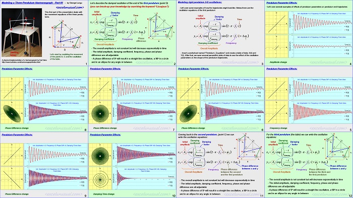
Hi guys, here is the first part of a tutorial describing the mathematical equations used in modeling a three-pendulum harmonograph (automatic drawing machine). It pertains to the second version of the model.
This section refers only to the kinematic equations for the movement of three pendulums. A second section will be published later and it will describe the kinematic equations involved in the articulated linkage mechanism on the top of the table, the custom spreadsheet functions used in the model and some overall considerations about the partition of the spreadsheet and the calculations going on in the workbook and VBA.
This is an advanced tutorial so you need a minimum of high-school physics and geometry background. Please tell us your views.
Modeling a Three-Pendulum Harmonograph – Part #1
by George Lungu
This first part of the presentation deals with the movement equations of the three pendulums.
Let’s start by modeling the movement of the points D, C and the oscillation of the table.
(Writing table)
A physical implementation of a harmonograph by Karl Sims
https://www.karlsims.com/harmonograph/index.html
<excelunusual.com> 1
Let’s describe the damped oscillation of the end of the first pendulum (point D)
(you can brush-up your knowledge by searching the keyword “Lissajous”):
Initial amplitude
Damping factor
Time
Phase difference
Damping coefficient Frequency
Overall Amplitude
– The overall amplitude is not constant but will decrease exponentially in time
– The initial amplitude, damping coefficient, frequency, phase and phase difference are all adjustable
– A phase difference of 0o will result in a straight line oscillation, a 90o in a circle and in an ellipse for any angle in between
<excelunusual.com>2
Modeling rigid pendulum 2-D oscillations:
– Let’s see some examples of how the trajectories might look like. Below there are the oscillation equations of the first pendulum.
Initial amplitude
Damping factor
Time
Damping coefficient
Frequency
Overall Amplitude
– Insert a worksheet named “Pendulum_Equations” and create a table of data: X(t) and Y(t). After that, we save several parametric plots of
data to see the effect of the oscillation parameters on the shape of the pendulum trajectories.
<excelunusual.com> 3
Pendulum Parameter Effects:
– Let’s see several examples of effects of pendulum parameters on pendulum end trajectories:
Amplitude change
<excelunusual.com> 4
Pendulum Parameter Effects (continuation):
Frequency change
<excelunusual.com> 5
Pendulum Parameter Effects (continuation):
Init. Amplitude=1.2, Frequency=5, Phase Diff.=0, Damping Time=2sec.
0.7 0.5
Time [s]
0.2 0
0 0.5 1 1.5 2 2.5 3 3.5 4 4.5 5
Init. Amplitude=1.2, Frequency=10, Phase Diff.=60, Damping Time=2sec.
0.7 0.5
Time [s]
0.2 0
X 0 0.5 1 1.5 2 2.5 3 3.5 4 4.5 5
-1.5 -1 -0.5 0 0.5 1 1.5
-0.3 -0.5
X(t)
-0.8 -1 Y(t)
-1.3 -1.5
Phase Difference change
<excelunusual.com> 6
Pendulum Parameter Effects (continuation):
1.7 1.5
Init. Amplitude=1.2, Frequency=5, Phase Diff.=0, Damping Time=2sec.
1.2 1
0.7 0.5
Time [s]
0.2 0
X 0 0.5 1 1.5 2 2.5 3 3.5 4 4.5 5
-1.5 -1 -0.5 0 0.5 1 1.5
-0.3 -0.5
X(t)
-0.8 -1
Y(t)
Init. Amplitude=1.2, Frequency=10, Phase Diff.=90, Damping Time=2sec.
1.2 1
0.7 0.5
Time [s]
0.2 0
X 0 0.5 1 1.5 2 2.5 3 3.5 4 4.5 5
-1.5 -1 -0.5 0 0.5 1 1.5
-0.3 -0.5
X(t)
-0.8 -1 Y(t)
-1.3 -1.5
Phase Difference change
<excelunusual.com> 7
Pendulum Parameter Effects (continuation):
1.7 1.5
Init. Amplitude=1.2, Frequency=5, Phase Diff.=0, Damping Time=2sec.
1.2 1
0.7 0.5
Time [s]
0.2 0
X 0 0.5 1 1.5 2 2.5 3 3.5 4 4.5 5
-1.5 -1 -0.5 0 0.5 1 1.5
-0.3 -0.5
X(t)
-0.8 -1
Y(t)
-1.3 -1.5
1.7 1.5
Init. Amplitude=1.2, Frequency=10, Phase Diff.=135, Damping
1.2 1
Time=2sec.
0.7 0.5
Time [s]
0.2 0
X 0 0.5 1 1.5 2 2.5 3 3.5 4 4.5 5
-1.5 -1 -0.5 0 0.5 1 1.5
-0.3 -0.5
X(t)
-0.8 -1
Y(t)
-1.3 -1.5
Phase Difference change
<excelunusual.com> 8
Pendulum Parameter Effects (continuation):
1.7 1.5
Init. Amplitude=1.2, Frequency=5, Phase Diff.=0, Damping Time=2sec.
1.2 1
0.7 0.5
Time [s]
0.2 0
X 0 0.5 1 1.5 2 2.5 3 3.5 4 4.5 5
-1.5 -1 -0.5 0 0.5 1 1.5
-0.3 -0.5
X(t)
-0.8 -1
Y(t)
-1.3 -1.5
1.7 1.5
Init. Amplitude=1.2, Frequency=10, Phase Diff.=180, Damping
1.2 1
Time=2sec.
0.7 0.5
Time [s]
0.2 0
X 0 0.5 1 1.5 2 2.5 3 3.5 4 4.5 5
-1.5 -1 -0.5 0 0.5 1 1.5
-0.3 -0.5
X(t)
-0.8 -1
Y(t)
-1.3 -1.5
<excelunusual.com> 9
Pendulum Parameter Effects (continuation):
1.7 1.5
Init. Amplitude=1.2, Frequency=10, Phase Diff.=90, Damping Time=2sec.
1.2 1
0.7 0.5
Time [s]
0.2 0
X 0 0.5 1 1.5 2 2.5 3 3.5 4 4.5 5
-1.5 -1 -0.5 0 0.5 1 1.5
-0.3 -0.5
X(t)
-0.8 -1
Y(t)
-1.3 -1.5
1.7 1.5
Init. Amplitude=1.2, Frequency=10, Phase Diff.=90, Damping
1.2 1
Time=0.3sec.
0.7 0.5
Time [s]
0.2 0
X 0 0.5 1 1.5 2 2.5 3 3.5 4 4.5 5
-1.5 -1 -0.5 0 0.5 1 1.5
-0.3 -0.5
X(t)
-0.8 -1 Y(t)
-1.3 -1.5
Damping Time change
<excelunusual.com> 10
Coming back to the second pendulum, (point C) we can write the oscillation equations: 2
Damping E
Initial Damping x
coefficient
amplitude factor
Time
2 2 2 2 1
damping A
osc(t) = y *A * exp * sin ( 2 *a* f *t)/b
2 2 2 2 2
damping
Phase difference between x and y
Frequency Phase difference
Overall Amplitude between the second and the first pendulum.
– The overall amplitude is not constant but will decrease exponentially in time
– The initial amplitude, damping coefficient, frequency, phase and phase difference are all adjustable
– A phase difference of 0o will result in a straight line oscillation, a 90o in a circle and in an ellipse for any angle in between
<excelunusual.com> 11
C
For the third pendulum (the table) we can write the oscillation
y
equations: 2
B
Damping E
Initial Damping x
2
coefficient
amplitude factor
Time
Damping factor
Phase difference
between x and y
Frequency Phase difference
Overall Amplitude between the third and the first pendulum
– The overall amplitude is not constant but will decrease exponentially in time
– The initial amplitude, damping coefficient, frequency, phase and phase difference are all adjustable
– A phase difference of 0o will result in a straight line oscillation, a 90o in a circle and in an ellipse for any angle in between
by George Lungu <excelunusual.com>


