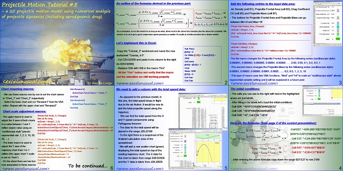
This is the next in a series of projectile motion tutorials for creating 2D trajectory models using numerical analysis of projectile dynamics (including aerodynamic drag).
The trajectory formulas were derived in the previous tutorial.
This post describes the Excel implementation (spreadsheet formulas, VBA code, buttons and charts).
Projectile Motion Tutorial #5 – a 2D projectile motion model using numerical analysis of projectile dynamics (including aerodynamic drag)
by George Lungu <excelunusual.com>
An outline of the formulas derived in the previous part:
As a conclusion, to run this model for as long as we want, all we need is the above four formulas plus the above ten constants.
We choose t so as to get a good compromise speed-precision (a smaller Dt results in a better precision but a slower model).
Let’s implement this in Excel:
-Copy the “Tutorial_3” worksheet and name the new worksheet “Tutorial_4-5”
-Cut C25:G2200 and paste it one column to the right (to D25:H2200)
-Replace G36 with H36 in the macro “Fire”
-Hit the “Fire” button and verify that the macro and the animation are still working properly
Sub Fire()
[B20] = 0
Do While [G36] > 0 And [B20] < 2000
DoEvents
[B20] = [B20] + 1LoopSleep 1000[B20] = 0
Exit Sub
End Sub
<excelunusual.com> 2
Add the following entries to the input data area:
-Air Density (cell B1), Projectile Frontal Area (cell B3), Drag Coefficient
CX (cell B5) and Projectile Mass (cell B7)
– The buttons for Projectile Frontal Area and Projectile Mass can go
between Min=0 and Max=18
Private Sub Frontal_Area_Change()
arrScale = Array(1, 2, 5)
[B3] = arrScale(Frontal_Area.Value Mod 3) * 10 ^ Int(Frontal_Area.Value / 3) / 1000000
End Sub
——————————————————————————————————————
Private Sub Mass_Change()
arrScale = Array(1, 2, 5)
[B7] = arrScale(Mass.Value Mod 3) * 10 ^ Int(Mass.Value / 3) / 100000
End Sub
-The fist macro changes the Projectile Frontal Area by the following series (oscilloscope style):
0.000001, 0.000002, 0.000005. 0.00001, 0.00002…….0.02, 0.05, 0.1, 0.2, 0.5, 1
– The second macro changes the Projectile Mass by the following series (oscilloscope style):
0.00001, 0.00002, 0.00005. 0.0001, 0.0002… 0.2, 0.5, 1, 2, 5, 10
– This type of macro uses two VBA functions, “Mod” and “Int” to crate an “oscilloscope style” almost
exponential variable setting and it will be explained in a future post
<excelunusual.com> 3
The initial conditions:
– The cells you can see to the right with text in the highlighted
areas are just labels
– After filling in for labels let’s input the initial conditions:
– Cell B26: “=B10*COS(RADIANS(B12))”
– Cell C26: “=B10*SIN(RADIANS(B12))”
– Cell D26: “=0”, Cell E26: “=B14”
Here are the formulas (from page 2 of the current presentation):
previous x previous_ y
-Cell B27: “=B26*(1-B$1*B$3*B$5
current x previous_ x
*SQRT(B26^2+C26^2)*B$16/(2*B$7))”
previous x previous_ y
Cell C27: “=C26*(1-B$1*B$3*B$5*
current_ y previous_ y
SQRT(B26^2+ C26^2)*B$16/(2*B$7))-
9.81*B$16”
current previous current_ y
– Cell E27: “=E26+C27*$B$16”
– After entering the above formulas copy down the range B27:E27 to row 2100
<excelunusual.com>4
We need to add a column with the total speed data:
– As opposed to the previous model, in
this one, the total speed drops in flight
due to the air friction. It would be nice to
plot the total projectile speed along the
trajectory
– We can find the total speed from the X
and Y speed components using
Pythagoras theorem
– The data for the total speed will be
placed in the range J26:J2100
– To the right there is a snapshot of the
finalized calculation area of the
spreadsheet
– We will add a new scatter chart (green)
displaying the total speed on top of the
existing trajectory chart. The X data for
this chart is taken from range D26:D2026
and the Y data is taken from J26:J2026
<excelunusual.com> 5
Chart renaming macros:
-We use these macros one by one to set the chart names to “Chart_1” and “Chart_2” respectively
-Select the lower chart and run “Rename1” from the VBA editor, Repeat with the upper chart and “Rename2”
Sub Rename1()
ActiveChart.Parent.Name = “Chart_1”
End Sub
Sub Rename2()
ActiveChart.Parent.Name = “Chart_2”
End Sub
Chart scale adjustment macros:
-The upper macro is used to adjust the X axes of both charts to a value between 1 and 1 million (same value using an “oscilloscope style” pseudo exponential rule: 1, 2, 5, 10, 20, 50, …)
-The lower macro is used to adjust the Y axis of the trajectory chart from 1 to 1 million (the upper chart Y scale is set on “Auto”)
-On the sheet there are two but-tons associated to these macros
Private Sub Scale_X_Change()
Dim aX As LongarrScale = Array(1, 2, 5)
aX = arrScale(Scale_X.Value Mod 3) * 10 ^ Int(Scale_X.Value / 3)
ActiveSheet.ChartObjects(“Chart_1”).Chart.Axes(xlCategory).MaximumScale = aX
ActiveSheet.ChartObjects(“Chart_2”).Chart.Axes(xlCategory).MaximumScale = aX
End Sub
Private Sub Scale_Y_Change()
Dim aX As LongarrScale = Array(1, 2, 5)
aY = arrScale(Scale_Y.Value Mod 3) * 10 ^ Int(Scale_Y.Value / 3)
With ActiveSheet.ChartObjects(“Chart_1”).Chart
.Axes(xlValue).MinimumScale = 0
.Axes(xlValue).MaximumScale = aY
End With
End Sub
To be continued…
by George Lungu <excelunusual.com>


