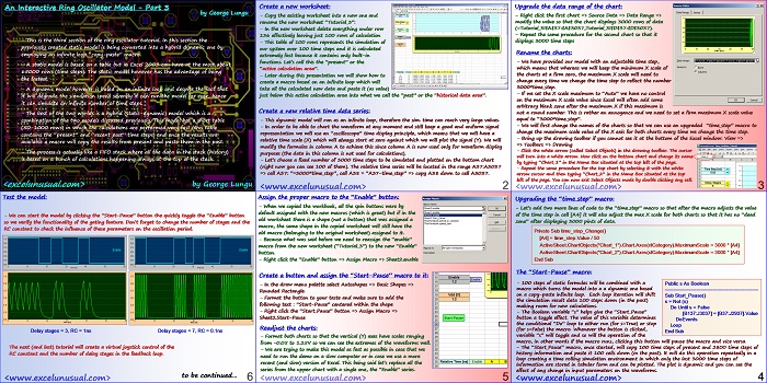
This is the third part of tutorial about making an interactive animated Excel model of a gated ring oscillator in MS Excel 2003.
This section deals with upgrading the model from a static table based one (with only 800 time steps) to a hybrid static-dynamic which is reasonably fast, yet it can run for an indefinite number of time steps.

An Interactive Ring Oscillator Model – Part 3
by George Lungu
– This is the third section of the ring oscillator tutorial. In this section the
previously created static model is being converted into a hybrid dynamic one by
employing an infinite loop “copy-paste” macro.
– A static model is based on a table but in Excel 2003 can have at the most about
65000 rows (time steps). The static model however has the advantage of being
the fastest.
– A dynamic model however is based on an infinite loop and despite the fact that
it will degrade the simulation speed severely it can run the model for ever, hence
it can simulate an infinite number of time steps.
– The best of the two worlds is a hybrid (static-dynamic) model which is a
combination of the two models discussed previously. This model has a short table
(50-1000 rows) in which the calculations are performed very fast (this table
contains the “present” and “recent past” time steps) and once the results are
available a macro will copy the results from present and paste them in the past.
– The process is actually like a FIFO stack where all the data in the stack (history)
is based on a bunch of calculations happening always at the top of the stack.
<excelunusual.com> by George Lungu
Create a new worksheet:
– Copy the existing worksheet into a new one and
rename the new worksheet “Tutorial_3”:
– In the new worksheet delete everything under row
136 effectively leaving just 100 rows of calculation
– This table of 100 rows represents the simulation of
our system over 100 time steps and it is calculated
extremely fast because it contains only built-in
functions. Let’s call this the “present” or the
“active calculation area”.
– Later during this presentation we will show how to
create a macro based on an infinite loop which will
take all the calculated new data and paste it (as value)
just below this active calculation area into what we call the “past” or the “historical data area”.
Create a new relative time data series:
– This dynamic model will run as an infinite loop, therefore the sim. time can reach very large values.
– In order to be able to chart the waveform at any moment and still keep a good and uniform signal
representation we will use an “oscilloscope” time display principle, which means that we will have a
relative time scale (X) which will always start at zero against which we will plot the signal (Y). We will
modify the formulas in column A to achieve this since column A is now used only for waveform display
purposes (the data in this column is not used for calculations).
– Let’s choose a fixed number of 3000 time steps to be simulated and plotted on the bottom chart
(right now you can see 100 of them). The relative time series will be located in the range A37:A3037
=> cell A37: “=3000*time_step”, cell A38 = “A37-time_step” => copy A38 down to cell A3037.
<excelunusual.com> 2
Upgrade the data range of the chart:
– Right click the first chart => Source Data => Data Range =>
modify the value so that the chart displays 3000 rows of data
(=Tutorial_3!$A$37:$A$3037,Tutorial_3!$D$37:$D$3037).
– Repeat the same procedure for the second chart so that it
displays 3000 time steps
Rename the charts:
– We have provided our model with an adjustable time step,
which means that whereas we will keep the minimum X scale of
the charts at a firm zero, the maximum X scale will need to
change every time we change the time step to reflect the number
3000*time_step.
– If we set the X scale maximum to “Auto” we have no control
on the maximum X scale value since Excel will often add some
arbitrary blank zone after the maximum X if this maximum is
not a round number. This is rather an annoyance and we need to set a firm maximum X scale value
equal to “3000*time_step”.
– We will first change the names of the charts so that we can use an upgraded “time_step” macro to
change the maximum scale value of the X axis for both charts every time we change the time step.
– Bring up the drawing toolbar if you cannot see it at the bottom of the Excel window: View =>
=> Toolbars => Drawing
– Click the white arrow (called Select Objects) in the drawing toolbar. The cursor
will turn into a white arrow. Now click on the bottom chart and change its name
by typing “Chart_1” in the Name Box situated at the top left of the page.
– Repeat the same procedure for the top chart by selecting it with the white
arrow cursor and then typing “Chart_2” in the Name Box situated at the top
left of the page. You can now exit Select Objects mode by double clicking any cell.
<excelunusual.com> 3
Upgrading the “time_step” macro:
– Let’s add two more lines of code to the “time_step” macro so that after the macro adjusts the value
of the time step in cell [A4] it will also adjust the max X scale for both charts so that it has no “dead
zone” after displaying 3000 pints of data.
Private Sub time_step_Change()
[A4] = time_step.Value / 50
ActiveSheet.ChartObjects(“Chart_1”).Chart.Axes(xlCategory).MaximumScale = 3000 * [A4]
ActiveSheet.ChartObjects(“Chart_2”).Chart.Axes(xlCategory).MaximumScale = 3000 * [A4]
End Sub
The “Start-Pause” macro:
– 100 steps of static formulas will be combined with a Public s As Boolean
macro which turns the model into a a dynamic one based
———————————————————
on a copy-paste infinite loop. Each loop iteration will shift
Sub Start_Pause()
the simulation result data 100 steps down (in the past)
s = Not (s)
making room for new calculations.
Do Until s = False
– The Boolean variable “s” helps give the “Start_Pause”
[B137:J3037] = [B37:J2937].Value
button a toggle effect. The value of this variable determines
DoEvents
the conditional “Do” loop to either run (for s=True) or stop
Loop
(for s=False) the macro. Whenever the button is clicked,
End Sub
variable “s” will toggle and so will the operation of the
macro, in other words if the macro runs, clicking this button will pause the macro and vice versa.
– The “Start_Pause” macro, once started, will copy 100 time steps of present and 2800 time steps of
history information and paste it 100 cells down (in the past). It will do this operation repeatedly in a
loop creating a time rolling simulation environment in which only the last 3000 time steps of
information are stored in tabular form and can be plotted. The plot is dynamic and you can see the
effect of any change in input parameters on the waveforms.
<excelunusual.com> 4
Assign the proper macro to the “Enable” button:
– When we copied the workbook, all the spin buttons were by
default assigned with the new macros (which is great) but if in the
old worksheet there is a shape (not a button) that was assigned a
macro, the same shape in the copied worksheet will still have the
old macro (belonging to the original worksheet) assigned to it.
– Because what was said before we need to reassign the “enable”
macro from the new worksheet (“Tutorial_3”) to the new “Enable”
button.
– Right click the “Enable” button => Assign Macro => Sheet2.enable
Create a button and assign the “Start-Pause” macro to it:
– In the draw menu palette select Autoshapes => Basic Shapes =>
Rounded Rectangle.
– Format the button to your taste and make sure to add the
following text : “Start-Pause” centered within the shape
– Right click the “Start_Pause” button => Assign Macro =>
Sheet2.Start-Pause
Readjust the charts:
– Format both charts so that the vertical (Y) axes have scales ranging
from -0.05 to 1.25V so we can see the extremes of the waveforms well.
– We are trying to make this model as fast as possible in case that we
need to run the demo on a slow computer or in case we use a more
recent (and slow) version of Excel. This being said let’s replace all the
series from the upper chart with a single one, the “Enable” series.
<excelunusual.com> 5
Test the model:
– We can start the model by clicking the “Start-Pause” button the quickly toggle the “Enable” button
so we verify the functionality of the gating feature. Don’t forget to change the number of stages and the
RC constant to check the influence of these parameters on the oscillation period.
1.15 1.15
0.95 0.95
0.75 0.75
Enable Enable
0.55 0.55
0.35 0.35
0.15 0.15
-0.05 -0.05
0 10 20 30 40 50 60 0 10 20 30 40 50 60
time [ns] time [ns]
1.15 1.15
0.95 0.95
0.75 0.75
0.55 0.55
0.35 0.35
0.15 0.15
-0.05 -0.05
0 10 20 30 40 50 60 0 10 20 30 40 50 60
time [ns] time [ns]
Delay stages = 3, RC = 1ns Delay stages = 7, RC = 0.1ns
The next (and last) tutorial will create a virtual joystick control of the
RC constant and the number of delay stages in the feedback loop.
to be continued…
<excelunusual.com> 6

