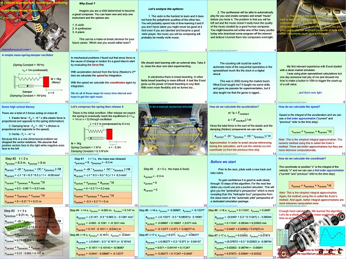
Here is the first part of a casual tutorial in both elementary dynamics and numerical methods.
It is written at a very basic level and it shows you how to solve a system of difference equations with a pencil and a paper and perhaps a pocket calculator to speed things up.
![]()
A casual approach to numerical modeling – the Spring-Mass-Damper-System – part 1.
by George Lungu @ <excelunusual.com>
Why Excel ?
Imagine you are a child determined to become a great composer. You can learn one and only one
instrument and the options are:
1. A violin
2. A synthesizer
3. A piano
This can be a make-or-break decision for your future career. Which one you would rather learn?
<excelunusual.com> 2
Let’s analyze the options:
1. The violin is the hardest to learn and it does not have the polyphonic qualities of the other two.
You will probably spend lots of time learning it and if you don’t have talent you might never be good at it.
And even if you are talented and became a good violin player, the music you will be composing will
probably be mostly violin music.
<excelunusual.com> 3
2. The synthesizer will be able to automatically play for you and create complex and smart “music”
before you know it. The problem is that you will be left out and the music doesn’t really have the quality
of the music created by a good human composer.
You might become not unlike one of the many youths today who download some program off the internet
and believe it turned them into composers overnight.
<excelunusual.com> 4
3. The piano is the right choice. It is not too hard to learn, yet hard enough that will force you to
understand music. And the range or styles you can compose using a piano is very large. Once you are a
good player you can augment your suite of tools with other instruments (such as a synthesizer).
My first relevant experience with Excel started with a stock market simulator.
I was using plain spreadsheet calculations but one day someone had pity of me and showed me
how to make a button in VBA to trigger the count-up of a cell value.
…and there was light.
<excelunusual.com> 6
The counting cell could be used to automate most of the sequential operations in the spreadsheet much like
the clock in a digital circuit.
This was in 2003 during the market boom.
What Excel taught me? It taught me some skills and gave me passion for experimentation, but it also taught me
that the game is rigged…
<excelunusual.com> 7
We should start learning with an external idea. Take it in, close the door and start experimenting.
In electronics there is bread boarding. In other fields bread boarding is more difficult. A tool like Excel
gives us the power of bread boarding in any field.
With even more flexibility and no fumes too…
<excelunusual.com> 8
In mechanical problems I found out that since force is the cause of change in motion it’s a good idea to start
by evaluating the force first. With acceleration derived from the force (Newton’s 2nd law) we calculate the speed by integration.
With the speed we calculate the coordinates again by integration.
We do all of these steps for every time interval and hope to get the right result…
<excelunusual.com> 9
A simple mass-spring-damper oscillator
(Spring Constant = 1N*m)
L0 = 1m (unstressed)
M = 1Kg
(Mass)
Damper
x = 0
(Damping Constant = 1N*s/m)
<excelunusual.com> 10
Some high school theory:
There are a total of 3 forces acting on mass M:
1. Elastic force : Fe = – K * x (the elastic force is proportional and opposite to the spring deformation)
2. Damping force : Fd = – DC * v (friction is proportional and opposite to the speed)
3. Inertia : Fi = – m * a
Because this is a one-dimensional problem we dropped the vector notations. We assume that positive
vectors face to the right while negative ones face to the left.
<excelunusual.com> 11
Let’s compress the spring then release it:
These is the initial condition. After release we expect the spring to eventually reach the equilibrium (L= L0
= 1m or x = 0) through oscillation
L = 0.7 m (compressed by 0.3 m)
M = 1Kg
Spring Constant = 1 N*m x = – 0.3m
Damping Constant = 0.3 N*s/m
<excelunusual.com> 12
Now let’s do a manual numerical simulation:
Let’s make some French Fries?
Slice the time domain in equally spaced intervals, say: Dt = 1 second apart
For each time slice repeat the same series of calculations:
a) Acceleration -> b) Speed -> c) Coordinate
How do we calculate the acceleration?
m *a = Fresultant
a = (Fresultant) / m
Since the total force is the sum of the elastic and the damping (friction) components we can write:
acurrent = -(K * xprevious + DC * vprevious ) / m
Approximation: In order to avoid circular referencing during this calculation, we’ll use the velocity (v) and coordinate (x) from the previous time step
<excelunusual.com> 14
How do we calculate the speed?
Speed is the integral of the acceleration and we can use a first order approximation (“current” and “previous” refer to the time step):
vcurrent = vprevious + acurrent *Dt
Note: This is the simplest integral approximation. The numeric method using this is called the Euler’s
method. There are better approximations but they are more intensive computationally.
<excelunusual.com> 15
How do we calculate the coordinate?
The coordinate or position “x” is the integral of the velocity “v” and we can use a first order approximation (“current” and “previous” refer to the time step):
xcurrent = xprevious + vcurrent *Dt
Note: This is the simplest integral approximation.
Again, the method using this is called the Euler’s method. And again, better integral approximations are more intensive computation wise.
<excelunusual.com> 16
Before we start:
Prior to the race, pilots walk a new track and take notes.
To gain confidence it is good to walk slowly through 10 steps of the algorithm.
For the next few slides you could use just a pocket calculator. This will give you the “pedestrian’s perspective” which is more
revealing than the “helicopter tour” perspective from the class room or the “automatic pilot” perspective of a dedicated simulation package.
<excelunusual.com> 17
Step #0 (t = 0 s, the mass is fixed)
xcurrent = – 0.3 m
vcurrent = 0
acurrent = 0
<excelunusual.com> 18
Step #1 t = 1 s, the mass was released
vprevious = 0, xprevious = – 0.3 m
acurrent = -(K * xprevious + DC * vprevious ) / M
0.3 m/s2
acurrent = -(-1 * 0.3 + 0.3 * 0 ) / 1 =
vcurrent = vprevious + acurrent *Dt
vcurrent = 0 + 0.3 *1 = 0.3 m/s
xcurrent = xprevious + vcurrent *Dt
xcurrent = -0.3 + 0.3 *1 = 0 m
<excelunusual.com> 19
Step #2 t = 2 s
vprevious = 0.3 m, xprevious = 0 m
acurrent = -(K * xprevious + DC * vprevious ) / M
-0.09 m/s2
acurrent = -(-1 * 0 + 0.3 * 0.3 ) / 1 =
vcurrent = vprevious + acurrent *Dt
vcurrent = 0.3 – 0.09 *1 = 0.21 m/s
xcurrent = xprevious + vcurrent *Dt
xcurrent = 0 + 0.21 *1 = 0.21 m
<excelunusual.com> 20
Step #3 t = 3 s
vprevious = 0.21 m, xprevious = 0.21 m
acurrent = -(K * xprevious + DC * vprevious ) / M
-0.273 m/s2
acurrent = -( 0.21+0.3 * 0.21 )=
vcurrent = vprevious + acurrent *Dt
vcurrent = 0.21 – 0.273 = – 0.063 m/s
xcurrent = xprevious + vcurrent *Dt
xcurrent = 0.21 – 0.063 = 0.147 m
<excelunusual.com>
Step #4 : t =4 s, vprevious = -0.063 m, xprevious = 0.147 m
acurrent = -( 0.147 -0.3 * 0.063 )= -0.1281 m/s2
vcurrent = -0.063 – 0.1281 = -0.1911 m/s
xcurrent = 0.147 – 0.1911 = -0.0441 m
Step #5: t =5 s, vprevious= -0.1911, xprevious= -0.0441
acurrent = -(-0.0441 -0.3 * 0.1911 )= 0.10143
vcurrent = -0.1911 + 0.10143 = -0.08967
xcurrent = -0.0441 – 0.08967 = -0.13377
<excelunusual.com>
Step #6 : t =6 s, vprevious = -0.08967, xprevious = -0.13377
acurrent = -(-0.13377 -0.3 * 0.08057)= 0.16067
vcurrent = -0.08967 + 0.16067 = 0.071 m/s
xcurrent = -0.13377 + 0.071 = -0.06277 m
Step #7: t =7 s, vprevious= 0.071, xprevious= -0.06277
acurrent = -(-0.06277 + 0.3 * 0.071 )= 0.04147
vcurrent = 0.071 + 0.04147 = 0.11247
xcurrent = -0.06277 + 0.11247 = 0.0497
<excelunusual.com>
Step #8 : t =6 s, vprevious = 0.11247, xprevious = 0.0497
acurrent = -(0.0497 + 0.3 * 0.11247) = -0.08344
vcurrent = 0.11247 – 0.08344 = 0.02903 m/s
xcurrent = 0.0497 + 0.02903 = 0.07873 m
Step #7: t =7 s, vprevious= 0.02903, xprevious= 0.07873
acurrent =-(0.07873 + 0.3 * 0.02903 )= -0.08744
vcurrent = 0.02903 – 0.08744 = – 0.05841
xcurrent = 0.07873 – 0.05841 = 0.02032
<excelunusual.com> 24
Enough hand calculations. We learned the algorithm.
Let’s do a check and plot the mass coordinate versus time as an Excel scatter plot:
0.3, 0.2
Time x
time [s]
Bingo! The mass seems to follow a damped oscillation towards the equilibrium point (what we expected).
by George Lungu <excelunusual.com>


