How to Model a Frequency Modulated (FM) Signal – an insight

Both frequency and phase modulation are important not only in electronics but also in science and physics in general.

It seems like a trivial chore but when I first tried to model such a signal some time back I hit a hard wall.

Our minds easily understand kinematics concepts such as coordinate, speed, acceleration and the relations between them in real life situations, but phase, frequency and angular acceleration are not so intuitive.

I will use a simple analogy to show that modeling an FM wave is a bit delicate but by no means a difficult process for the one who understands it.

[sociallocker][/sociallocker]

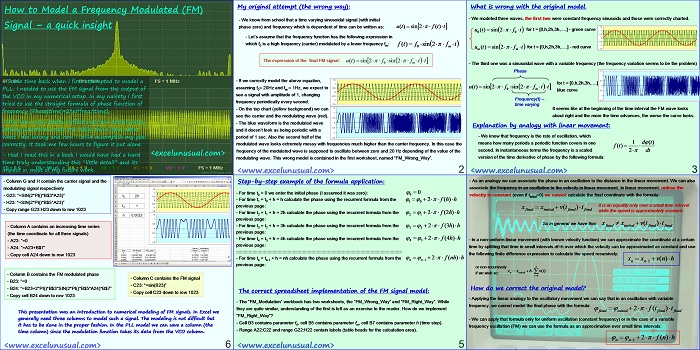
How to Model a Frequency Modulated (FM) Signal – a quick insight

by George Lungu

– Some time back when I first attempted to model a
PLL, I needed to use the FM signal from the output of
the VCO in my numerical setup.

In my naivety I first
tried to use the straight formula of phase function of
frequency [Phase(time)=2*pi*freq.*time].

-This had a very positive effect since the horrendously
looking waveform made me really think hard about
what I did wrong and how I could accomplish my goal
correctly.

It took me few hours to figure it out alone.
<excelunusual.com> – Had I read this in a book I would have had a hard
time truly understanding this “little detail” and its
impact in most of my future work.

My original attempt (the wrong way):

– We know from school that a time varying sinusoidal signal (with initial
phase zero) and frequency which is dependent of time can be written as: u(t)  sin  2    f (t)t

– Let’s assume that the frequency function has the following expression in
which f0 is a high frequency (carrier) modulated by a lower frequency fm: f(t) f sin  2  f t

– If we correctly model the above equation, assuming f0= 20Hz and fm = 1Hz, we expect to see a signal with amplitude of 1, changing frequency periodically every second.

– On the top chart (yellow background) we can see the carrier and the modulating wave (red).

– The blue waveform is the modulated wave and it doesn’t look as being periodic with a period of 1 sec. Also the second half of the -1.5
modulated wave looks extremely messy with frequencies much higher than the carrier frequency. In this case the
frequency of the modulated wave is supposed to oscillate between zero and 20 Hz depending of the value of the
modulating wave. This wrong model is contained in the first worksheet, named “FM_Wrong_Way”.

What is wrong with the original model?

– We modeled three waves, the first two were constant frequency sinusoids and those were correctly charted.

It seems like at the beginning of the time interval the FM wave looks
about right and the more the time advances, the worse the curve looks.

Explanation by analogy with linear movement:

– We know that frequency is the rate of oscillation, which
means how many periods a periodic function covers in one second. In instantaneous terms the frequency is a scaled version of the time derivative of phase by the following formula:

– As an analogy we can associate the phase in an oscillation to the distance in the linear movement. We can also
associate the frequency in an oscillation to the velocity in linear movement.

In linear movement, unless the
velocity is constant (even if t-initial=0) we cannot calculate the final coordinate with the formula:
it is an equality only over a small time interval while the speed is approximately constant.

So in general we have this: x +x +v(t )t

– In a non-uniform linear movement (with known velocity function) we can approximate the coordinate at a certain
time by splitting that time in small intervals dt=h over which the velocity can be approximated as constant and use
the following finite difference expression to calculate the speed recursively:
xn – x +v(n)*h
n1
or non-recursively
x -x +h* v(i)
n initial
if we wish so:
i+0

How do we correct the original model?

– Applying the linear analogy to the oscillatory movement we can say that in an oscillation with variable
frequency, we cannot model the final phase with the formula:

– We can apply that formula only for uniform oscillation (constant frequency) or in the case of a variable
frequency oscillation (FM) we can use the formula as an approximation over small time intervals:

Step-by-step example of the formula application:

– For time t0 = 0 we enter the initial phase (I assumed it was zero):

– For time t1 = t0 + h = h calculate the phase using the recurrent formula from the previous page

– For time t2 = t1 + h = 2h calculate the phase using the recurrent formula from the previous page

– For time t3 = t2 + h = 3h calculate the phase using the recurrent formula from the previous page

– For time t4 = t3 + h = 4h calculate the phase using the recurrent formula from the previous page

::::::::::::::::::::::::::::::::::::::::::::::::::::::::::::::::::::::::::::::::::::::::::::::::::::::::::::::::::::::::::::::::::::
– For time tn = tn-1 + h = nh calculate the phase using the recurrent formula from the previous page:

The correct spreadsheet implementation of the FM signal model:

– The “FM_Modulation_Tutorial” workbook has two worksheets, the “FM_Wrong_Way” and “FM_Right_Way”.
While they are quite similar, understanding of the first is left as an exercise to the reader. How do we
implement “FM_Right_Way”?

– Cell B3 contains parameter f0, cell B5 contains parameter fm, cell B7 contains parameter h (time step).

– Range A22:C22 and range G22:H22 contain labels (table heads for the calculation area).

– Column G and H contain the carrier signal and the
modulating signal respectively

– G23: “=SIN(2*PI()*B$3*A23)”

– H23: “=SIN(2*PI()*B$5*A23)”

– Copy range G23:H23 down to row 1023

– Column A contains an increasing time series (the time coordinate for all three signals)

– A23: “=0

– A24: “=A23+B$7”

– Copy cell A24 down to row 1023

– Column B contains the FM modulated phase

– Column C contains the FM signal

– B23: “=0

– C23: “=sin(B23)”

– B24: “=B23+2*PI()*B$3*SIN(2*PI()*B$5*A24)*B$7”

– Copy cell C23 down to row 1023

– Copy cell B24 down to row 1023

This presentation was an introduction to numerical modeling of FM signals. In Excel we
generally need three columns to model such a signal.

The modeling is not difficult but it has to be done in the proper fashion. In the PLL model we can save a column (the
time column) since the modulation function takes its data from the VCO column.

by George Lungu <excelunusual.com>