How to Model a Phase-Locked Loop (PLL) in Excel – part#1

A Phase-Locked Loop is a type of electronic circuit. It generates an oscillation with the same frequency as a reference oscillation and a relatively constant phase difference  with respect to the same reference. The applications spectrum of such a circuit are extremely wide.

Signal modulation, demodulation, detection and filtering, frequency conversion and synthesis are just a fraction of what this circuit can do.

Though very simple, it is often not enough understood in industry by people who use it or even design it.

This tutorial of a short series which uses the principles presented before in this blog, to casually model a basic PLL in Excel with minimum math.

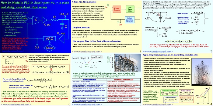
How to Model a PLL in Excel-part #1 – a quick and dirty, cook-book style recipe

by George Lungu

A phase locked loop (or a PLL) is an electronic circuit which generates a oscillatory output synchronized with an oscillatory input.

Just in telecommunications the PLL applications are very wide:

-signal synchronization

-signal recovery

-frequency synthesis

-signal demodulation

The first two presentations will NOT explain the PLL functionality in much detail, it will just explain the numerical method and show you how to implement your own fast and dynamic PLL model using minimum time and effort.

<excelunusual.com>

A basic PLL block diagram:

The general principle of a PLL is easy to understand:

-if the free running frequency of the voltage controlled oscillator is not too far from the input frequency any phase difference will be sensed by the phase detector, filtered and sent back to control the VCO frequency until the input and the output have exactly the same frequency and there is a constant phase difference between them.

The phase detector:

– Most of the written materials out there say that the phase detector is nothing more that an analog multiplier or a XOR gate in the digital case. In this presentation we will not try to understand why.

We will come back for more insight into this topic in future presentations.

For now we will just use a plain multiplication to model a phase detector in Excel.

 

The low pass filter (LPF) a basic difference derivation:

– This is a little bit more difficult to model so you need to pay attention. If you finally understand the derivation
of the numerical model you will be able to do much more complicated things by yourself.

Let’s not worry about filter theory and just pick a resistor and a capacitor and improvise a basic low pass filter.

Why is that circuit a LPF? Because for very low frequencies the capacitor has a large impedance and the signal
goes from input to output unchanged.

At very high frequencies the capacitor is a short, all the input signal is
grounded and the output is zero. For this circuit we can write (these formulas are high school level):
R, u (t), in, out
From Ohm’s law: R 
C
dq (t)
From the definition
u t C
t out =>
in of current intensity:
duout (t )
From the definition dq(t)
i(t)
of capacitance:
dt
Eliminate the u t)u (t)
in out
R 
dq (t )
current intensity:
R*dq( t)  u( t)u (t ) dt
in out
=> dt => =>
C*du( t)  dq (t )
dq (t) out
d_uout (t )
=> R*C*du (t)*u(t)*u (t)*dt
out in out

Don’t tell me you had any difficulties with the derivations on this page. If you did
you must go back to the high school physics book of problems and solve 100 of them.

 

Apply the previous formula on an elementary time step (dt):

– Numerical methods are very dumb but very efficient ways of solving very
difficult problems. We essentially calculate what happen on a very short time
interval.

Numerical methods are not exact methods, there are
approximations and intrinsic errors but the errors can be minimized by
choosing smaller time steps.

– Because the interval is so short, the laws of physics are simple and we can
often use linear approximations.

– Another factor that makes the numerical methods easy to work with is the
fact that we already know all the results from previous time steps and we can
use them to calculate the result of the current time step. It is all a recurrent
chain of calculations, just like the skyscraper builders who use no cranes but
use the previously build structure to attach the scaffolding on.

– Another very important factor in facilitating the calculations is the fact that
the derivatives (tangents) to curves of certain functions can be approximated
as secants, using the current and the previous value of the function.

f(t)
f(t+h)
Derivative definition: Central estimate:
To the right there are
three common derivative df (t) * f(t *dt)* f (t)* df (t) f(t*h)* f (t *h)

approximations which dt
dt * dt * dt 2*h
f(t-h)
dramatically simplify
Forward estimate: f(t)
calculations in numerical Backward estimate:
methods. Pay attention df (t ) f(t)*f (t *h)
df (t ) f(t* h)* f (t)

to colors.
dt h dt h
t-2h t-h t t+h t

t ,u (n),u (n)
n in out
t ,u (n-1),u (n-1)
n-1 in out
time
dt = h
t
n-2 t
t
n-1
In order to make the numerical methods easier to understand I set up an analogy with a
construction site. The analogy is somewhat idealistic. The construction methods described
here are quite unorthodox, devised purposely for this presentation.

Numerical Methods An Original Construction Site

Time domain – time step duration

Vertical dimension – floor height
Calculate one step at a time

– allows for handy approximations Build one floor at a time after completely finishing the floors and ease of calculations.

The previous time steps are fully underneath.

The workers and the machines are concentrated finished and their data can be displayed on a chart. on the current floor.

The floors underneath are in use.

Formulas and calculations are simple. Any enthusiastic geek

The workers have a solid and safe floor underneath. No need can program the methods instead of a employing a highly paid for hard to find “high iron” workers from Mohawk (part of
mathematician using a high price software. Iroquois) tribe.

Just about any worker will do the job since the skills to build within 10 feet of height are lower.

Calculations use only information from the previous 1-3 time

Instead of using an expensive crane workers just use steps. The scaffolding anchored to the previous 2-3 floors

For large simulation times, the model could be paused, storing

The construction crew could take a long vacation and restart the last 2-3 steps and it can be restarted from the same point the work any time with no major consequences while the any time later, after a day, a month or a year. The building underneath is in use.

Let’s see how by knowing everything about the previous time steps (up to time “n-1”) we can translate the above equation into a
numerical approximation equation with the purpose of finding the output voltage at the moment “n”:

The numerical equations to the left are equivalent and must give very close results. The former uses the backwards
approximation of the derivative and the latter uses the forward approximation.

The numerical output formula by
h_u (n)*R*C*u (n_1)
in out
u (n) 
out
backward derivative estimate:
R*C *h
The numerical output formula by h
u (n) *u (n_1)/u (n_1)*u (n_1)
out out in out
forward derivative estimate:
R*C
– Both formulas lead to the same result. The shorter the time step the better the precision of
either result. In the next section, before integrating the LPF formula into the PLL model, the
two formulas will be tried on a spreadsheet example using rectangular periodic signal as input.

– Whenever you build a model break it in simple stages and don’t proceed
to the next stage until you fully test the current stage.

to be continued…

by George Lungu <excelunusual.com>