This section of the turorial finalizes the main dynamics calculations and implements the numerical method for approximating the glider trajectory. At this point, the model is already functional but with a crude interface.
![]()

[sociallocker]![]() [/sociallocker]
[/sociallocker]
Longitudinal Aircraft Dynamics #10- the numerical method
by George Lungu
– This section deals worksheet implementation of the numerical setup for a dynamic modeling of
the flight. The model will already be functional by the end of this section.
An review of the method:
-We have both the x component and the y component of the resultant “present” force on the airplane
calculated from the “past” speeds and positions. We use the “present” force to calculate the “present”
x-y acceleration components (Newton’s second law). From acceleration we can calculate the “present”
speed components by integration and from speed we calculate the “present” x-y coordinates.
– We avoided calculating something from itself (circular referencing). A diagram of the method is shown
below:
Linear speed and coordinates (old) Angular speed and coordinate (old)
Gravity Aerodynamic extracted functions (lift force, drag force and pitching moment)
Moment
Mass Newton 2nd law (linear) Newton 2nd law (angular)
of inertia
Linear Acceleration Angular Acceleration
Integration Integration Integration Integration
Linear speed and coordinates (new) Angular speed and coordinate (new)
Numerical scheme implementation:
– Copy the last worksheet and name the new one “Longitudinal_ Stability_Model_6”
– There are three buttons, the “Reset”, the “Run_Pause” and the “CG_visibility” buttons. Make sure to
reassign the right macros to them, macros belonging to the current worksheet. By default, the custom
buttons (created by the user from a macro assigned shape) keep the macros from the original worksheet
assigned to them.
– We moved all the force and momenta calculation range near the input parameter buttons in order to
perform some testing. Let’s move them back to the original area: select range D19:E36 => Copy =>
select cell M66 => Paste.
– Copy the x and y force component to the present calculation area: B51: “=R77”, E51: “=R78”.
– Copy the pitching moment to the present calculation area: H51: “=R79”.
Speed calculation by the numerical integration of the linear acceleration:
– We will use the simplest approximation, a linear variation of the speed with time which means we assume that acceleration (hence force) is almost constant during
the duration of a simulation time step (the smaller the time step the better the approximation):
We will model the v v dt
present x past_ x
using Newton’s second m
problem separately law we write:
along the axes of a coordinates:
Coordinate calculation by the numerical integration of speed:
– Similarly we will use the simplest approximation, a linear variation of the coordinates with respect to time and just present past present_ x
like in the case of the speed approximation we can write present past present_ y
the numerical approximation of the linear coordinates:
Worksheet implementation:
– We can write the following formulas:
=> D51: “=D52+B51*Time_step/Mass”
=> E51: “=E52+C51*Time_step/Mass”
=> F51: “=F52+D51*Time_step”
=> G51: “=G52+E51*Time_step”
– In the snapshot to the right, the active (present)
formulas are on a green background and the “past” constant data is on an orange background.
Angular speed calculation by the numerical integration of the angular acceleration:
– Formally, the angular treatment is very similar to the linear dynamics treatment. The linear
acceleration (a) becomes angular acceleration (), dt d t
This says that the angular acceleration is equal
the linear speed (v) becomes angular speed (v) and
to the first derivative of angular speed with
linear coordinate (x) becomes angle or phase (J)
respect to time and also equal to the second
derivative of the angle with respect to time.
– There is even an angular form of Newton’s
moment of inertia
second law which says that the angular
moment angular acceleration is equal to the product between the acceleration
moment of inertia and the moment of force
Newton’s second law in angular form
– The formula for the moment of inertia of a uniform rod of mass and length “L” about its middle (center of mass – CM) is:
– Using the same procedure used for the derivation of the linear speeds and coordinates you can derive
the numerical approximation formulas for calculating the angular speed and the angular coordinate
(airplane angle) using the moment, the moment of inertia and the previous angular speeds and
coordinates. The proof is not given here, however you can see a side by side comparison of the linear
and angular formulas:
linear speeds force angular speeds
moment of force
F M
present x past_ x present past moment of inertia present past present_ x present past present
angles
linear coordinates
LINEAR ANGULAR
– It is interesting to notice that in our case we used “_plane” to denote the angle of the airplane
which in the above formula becomes theta (J).
– Another very important observation is that we have chosen as an input parameter the fractional
moment of inertia, which is the ratio of the moment of inertia of the plane divided with the moment
of inertia of a uniform rod having the same length and same mass as our airplane. For a glider I guess
a reasonable number would be around 0.3-0.5, since most of its mass is concentrated around the pilot
and the main wing.
– With the last notice in mind our final numerical equations become (see next page):
For ease of usage we expressed our present angles all over the model in degrees.
present past 2 The second formula includes a radians
fractional fuselage
to degrees conversion factor.
180 Conversion
_ planepresent _ plane v dt
past present from radians
to degrees
Worksheet implementation:
– We can write the following formulas:
=> I51: “=I52+(12*H51*Time_step)/
(Momentum_inertia*Mass*Length_fuselage^2)”
=> J51: “=J52+180*I51*Time_step/PI()”
– In the snapshot to the right, the active (present)
formulas are on a green background and the “past”
constant data is on an orange background.
Increasing the size of the historical trajectory data:
Sub Run_Pause()
runpause = Not (runpause)
– We provided a 1000 point long historical trajectory
Do While runpause = True
data (within the “Run_Pause()” and “Reset()” macros). We DoEvents
[D52:K3052] = [D51:K3051].Value
would like to increase that length let’s say to 3000.
Loop
– In order to do that let’s change the “Run_Pause()” and
End Sub
the “Reset()” macros as seen to the right.
– We can see that the macros are the same except for the Sub Reset()
size of the copied/pasted/cleared range. [D52:K3052].ClearContents
[D52:K52] = [D47:K47].Value
End Sub
Plotting the trajectory of the glider:
– Insert a 2D scatter chart with the range F51:F3051 as x-data and the range G51:G3051 as the
y-data. Also create a speed gauge:
0.2
M43: “=SQRT(D52^2+E52^2)”
Run the model:
– Adjust parameters, then => Reset => Run
-0.1 0.1 0.3 0.5 0.7 0.9
– If you see a lack of convergence (very large
numbers and the chart going haywire) reduce the
-0.2
size of the time step. For certain angles of attack,
60
beyond our modeling in Xflr 5 the model cannot
possible converge.
VICTORY !
50
– You cannot do loops yet. I am working on that
as we speak.
-300 -250 -200 -150 -100 -50 0
Three different glider trajectories for various launch conditions and CG positions.
-10
To be continued…