This brief tutorial explains how to calculate the solution vector of a system of linear equations using the Excel spreadsheet function MINVERSE() which calculate the inverse of a matrix.
![]()

[sociallocker]![]() [/sociallocker]
[/sociallocker]
Solving linear systems of equations in Excel – the easy way
by George Lungu
– This is a tutorial showing an easy and convenient method of solving moderate size systems of
linear equations in Excel by using the built-in formulas for matrix inversion, MINVERSE() and
matrix multiplication, MMULT().
– There are many different ways of solving such systems, a lot of this methods are studied in
school or college. This presentation will not deal with the theory of these methods or even
mentioning them. Whoever wants to learn more must do a Google search into “system of linear
equations”. Wikipedia has a good entry on this topic too.
We can turn the system of linear equations
previous system of equations in
with 3 unknowns
matrix equation:
looks like this: 3
and [B] is
Where [A] is the [X] is the matrix
the matrix
coefficient matrix: of unknowns:
of constants:
<excelunusual.com>
Solving the system of equations using the INVERSE matrix:
If we can find the inverse of the coefficient
matrix we can solve the matrix equation by
multiplying both sides of the equation with
the inverse of that matrix from the left side:
Using the associativity of matrix
multiplication we can write:
the identity matrix
Excel implementation example for a 3 x 3 system of linear equations:
– In an new worksheet input two
matrices as arrays of numbers: the
matrix of coefficients in the range
B3:D5 and the matrix of constants
in the range B10:B12.
– The formulas for calculating the
solution will be placed in range
D10:D12.
– You can use different labels and
colors if you wish so.
How to fill the solution matrix formula:
– Select cell D10, type “=MMULT(MINVERSE(B3:D5),B10:B12)” then hit return.
– Select range D10:D12 and press F2+Ctrl+Shift+Enter in this order.
– The solution vector should appear in the range D10:D12.
– If the system has no solution or infinite solutions, you will get the #NUM! error message in
the solution range. If you left a cell blank the result will be #VALUE! error message in the cells
of the result range.
Verify the result:
-Let’s calculate vector [B] from the solution backwards to confirm the correctness of the result:
=> D15: “=B3*D$10+C3*D$11+D3*D$12” then copy D15 down to cell D17
– Range D15:D17 will contain results equal to the numbers in the vector of constants [B] which
proves that the algorithm used for calculating the solution (in range D10:D12) is correct.
Calculate the result in a horizontal vector form:
– Sometimes it is useful to have the result as a horizontal vector and we
can get that using the function TRANSPOSE()
– Select cell B19 and type “=TRANSPOSE(MMULT(MINVERSE(B3:D5),
B10:B12))” then hit return.
– Select range B19:D19 and press F2+Ctrl+Shift+Enter in this order.
– The solution vector should appear in the range B19:D19.

It’s surprising to find on excelunusual.com a resource so precious about equations.
We will note your page as a benchmark for The Easy Way of Solving Systems
of Linear Equations in Excel – using the INVERSE() spreadsheet function.
We also invite you to link and other web resources for
equations like https://equation-solver.org/ or https://en.wikipedia.org/wiki/Equation.
Thank you ang good luck!