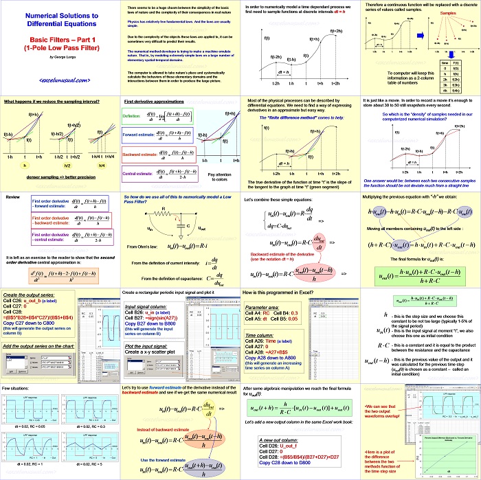
This post shows the steps for building a first model of a single pole RC low pass filter (LPF) in Excel based on numerical solution using the finite difference method.
It is quite easy to understand, try to go through the proof regardless of your background.
Basic Filters – Part 1 (1-Pole Low Pass Filter) – Numerical Solutions to Differential Equations (Finite Difference Method)
by George Lungu
Introduction:
There seems to be a chasm between the simplicity of the basic laws of nature and the complexity of their consequences in real nature
Physics has relatively few fundamental laws. And the laws are usually simple.
Due to the complexity of the objects these laws are applied to, it can be sometimes very difficult to predict their results.
The numerical method developer is trying to make a machine emulate nature. That is, by modeling extremely simple laws on a large number of elementary spatial-temporal domains.
The computer is allowed to take nature’s place and systematically calculate the behaviors of these elementary domains and the interactions between them in order to produce the large picture.
<excelunusual.com> 2
In order to numerically model a time dependent process we first need to sample functions at discrete intervals dt = h
f(t+2h)
f(t)
f(t+h)
f(t)
f(t-2h)
f(t-h)
dt = h
t-2h t-h t t+h t+2h
<excelunusual.com> 3
Therefore a continuous function will be replaced with a discrete series of values called samples.
Samples:
f(t+2h), f(t), f(t+h), f(t+2h), f(t+h), f(t), f(t-2h), f(t-h), f(t), f(t-2h), f(t-h), dt = h
t-2h t-h t t+h t+2h t-2h t-h t t+h t+2h
time F(t)
Te computer will keep this information as a 2-column table of numbers.
2h f(2h), 3h f(3h), 4h f(4h)
<excelunusual.com> 4
It is just like a movie. In order to record a movie it’s enough to store about 30 to 50 still snapshots every second.
So which is the “density” of samples needed in our computerized numerical simulation?
f(t+2h), f(t), f(t+h), f(t), f(t-2h), f(t-h)
dt = h
t-2h t-h t t+h t+2h
One answer would be: between each two consecutive samples the function should be not deviate much from a straight line.
<excelunusual.com> 5
Most of the physical processes can be described by differential equations. We need to find a way of expressing derivatives in an approximate but easy way.
The “finite difference method” comes to help:
This method approximates the tangent to the curve in point “t” (green curve) with something easy, much more convenient in calculation – the secant to the curve (there are three options available around point “t”)
f(t), f(t+h), f(t-h), f(t)
dt = h
t-2h t-h t t+h t+2h
<excelunusual.com> 6
First derivative approximations:
Definition: df (t) /dt=lim|dt->0[( f(t +dt )- f (t ))/dt]
Forward Estimate: df (t) /dt=( f(t + h )- f (t ))/h — where h->0
Backward Estimate: df (t) /dt=( f(t)- f (t – h ))/h — where h->0
Central Estimate: df (t) /dt=( f(t + h )- f (t – h))/(2*h) — where h->0
Pay attention to colors!
<excelunusual.com> 7
What happens if we reduce the sampling interval?
f(t+h)
f(t+h/2)
f(t)
f(t-h/2)
f(t-h)
f(t) f(t)
t-h t t+h t+ t-h/2 t t+h/2 t-h/4 t t+h/4
h h/2 h/4
denser sampling => better precision !!!
<excelunusual.com> 8
Review:
First order derivative – Forward Estimate:
— where h->0
First order derivative – Backward Estimate:
— where h->0
First order derivative – Central Estimate:
— where h->0
It is left as an exercise to the reader to show that the second order derivative central approximation is:
<excelunusual.com> 9
So how do we use all of this to numerically model a Low Pass Filter?
From Ohm’s law:
From current definition:
From capacitance definition:
<excelunusual.com> 10
Let’s combine these simple equations:
Combining the above equations:
Now we can use the backward estimate of the derivative:
<excelunusual.com> 11
Multiplying the previous equation with “-h” we obtain:
Moving all members containing u_out(t) to the left side :
The final formula for u_out(t) is:
<excelunusual.com> 12
h – this is the step size and we choose this constant to be not too large (typically 1-5% of the signal period)
u_int(t) – this is the input signal at moment “t”, we also choose this one as initial condition
RC- this is a constant and it is equal to the product between resistance and capacitance
u_out (t -h) – this is the previous value of the output and it out was calculated for the previous time step (u_out(0) is chosen as a constant – called an initial condition)
<excelunusual.com> 13
How is this programmed in Excel?
Open a new workbook, select the first worksheet (lower left bottom) and rename it “LPF_backward”
Parameter area:
Cell A4: RC Cell B4: 0.3
Cell A5: dt Cell B5: 0.05
Time column:
Cell A26: Time (a label)
Cell A27: 0
Cell A28: =A27+B$5
Copy A28 down to A800
(this will generate an increasing
time series on column A)
<excelunusual.com> 14
Create a rectangular periodic input signal and plot it:
Input signal column:
Cell B26: u_in (a label)
Cell B27: = sign(sin(A27))
Copy B27 down to B800
(this will generate the input series on column B)
Plot the input signal:
Create a x-y scatter plot
<excelunusual.com> 15
Create the output series:
Cell C26: u_out_b (a label)
Cell C27: 0
Cell C28: =(B$5*B28+B$4*C27)/(B$5+B$4)
Copy C27 down to C800
(this will generate the output series on column B)
Add the output series on the chart:
<excelunusual.com> 16
A few situations:
1.5 1.5
LPF response LPF response
1 1
0.5 0.5
time(s) time(s)
0 0
0 2 4 6 8 10 12 14 16 18 0 2 4 6 8 10 12 14 16 18
-0.5 -0.5
-1 -1
RC = 0.05 In Out RC = 0.3 In Out
-1.5 -1.5
dt = 0.02, RC = 0.05 dt = 0.02, RC = 0.3
1.5 1.5
LPF response LPF response
1 1
0.5 0.5
time(s) time(s)
0 0
0 2 4 6 8 10 12 14 16 18 0 2 4 6 8 10 12 14 16 18
-0.5 -0.5
-1 -1
RC = 1 In Out RC = 5 In Out
-1.5 -1.5
dt = 0.02, RC = 1 dt = 0.02, RC = 5
<excelunusual.com> 17
Let’s try to use forward estimate of the derivative instead of the backward estimate and see if we get the same numerical result:
Instead of backward estimate
Use the forward estimate
<excelunusual.com> 18
After some algebraic manipulation we reach the final formula for u_out(t):
-Make a copy the worksheet and rename it “LPF_back+forward”
– In this new worksheet do the following:
A new out column:
Cell D26: U_out_f
Cell D27: 0
Cell D28: =(B$5/B$4)/(B27+D27)+D27
Copy C28 down to D800
<excelunusual.com> 19
– We can see that the two output waveforms overlap!
– We can see that the two output waveforms overlap!
-Here is a plot of the difference between the two methods function of the time step size
by George Lungu <excelunusual.com>


This is just great, thanks for this!
existen otros casos de problemas de valores de frontera, en los cuales las series de Fourier, los casos de funciones periódicas en estado natural (como es el caso de su aplicación en medicina, los electrocardiogramas, se grafica el voltaje de la corriente electrica de los latidos del corazón)su ejemplo me recordó este método de ecuaciones diferenciales. involucran fuciones senoidales y cosenoidales:
acos(n*pi*t/t1)+b*sin(n*pi*t/t2)
su método me ayudará a poder graficarlos. thanks!. Vorwärts!