This is a first post of an introduction to optics series and it explain how to create a 2D ray tracing model for a spherical mirror.
This section deals with the creation and charting of the mirror using a parametric equation for a circle.
![]()

[sociallocker]![]() [/sociallocker]
[/sociallocker]
Introduction to Geometrical Optics – a 2D ray tracing Excel model for spherical mirrors – Part 1
by George Lungu
– This is a tutorial explaining the creation of an exact 2D ray tracing model for both
spherical concave and spherical convex mirrors.
– The model is 2D in the sense that the ray tracing is done in the median x-y plane of
symmetry of the mirror
– This is an exact model in the sense that no geometrical approximations are used, however
the model does not take into consideration diffraction effects.
The ideal reflection laws:
There are two reflection laws:
1. The incident ray the normal to the surface and
the reflected ray are situated in the same plane
2. The angle of incidence and the angle of
reflectance are equal
Creating the chart of a spherical mirror section:
– This being a 2D ray tracing program, the spherical
mirror will be represented by a section through its x-y
median plane which is a circular arc. R R*sin()
-We use a parametric Cartesian representation of the circular arc based on the definition of the trigonometric
functions on the trigonometric circle.
the angle being proportional to a parameter index
Conventions and Excel implementation:
– In our model the light will travel from left to right before the
reflection.
– By an ad-hoc convention the radius of the curvature will be positive
for a convex mirror and negative for a concave mirror
– Column A will contain labels.
– Parameters xM and yM are the position of the vertex of the mirror
and are located in range B2:B3. We name cell B2 “xM” and B3 “yM”.
– The radius is placed in cell B4 and we name that cell “Radius”
– Cell B5 contains the diameter of the mirror and we name that cell
“d”
– Cell B6 contains the length of the hachured area behind the
reflective surface and we name the cell “Back”
Creating the spherical mirror:
– Range A42:A62 will contain the index parameter which will
have the function of scanning a mirror angle (measured from the
center of curvature) starting with the top (d/2) of the mirror
and ending with the bottom (-d/2) in 21 steps.
– While increment “i” varies from -10 to 10 in increments of 1
the (x,y) coordinates described in the formulas above will trace an
arc of circle with a size (length) of “d”, the radius of “Radius”,
and the vertex placed at coordinate (xM,yM) then copy A42 down to A62
– B42: “=Radius*(1-COS((A42/10)*ASIN(d/(2*Radius)))) +xM” then copy
B42 down to cell B62
– C42: “=Radius*SIN((A42/10)*ASIN(d/(2*Radius)))+yM” then copy C42
down to cell C62
Chart the mirror:
– Select rage B42:C62 => Insert => Chart =>
Scatter Chart => Finish => delete the legend
– Right click the horizontal axis => Format
Axis => Scale => Minimum=-5, Maximum=5,
Max Unit=1, Min Unit=1
– Right click the vertical axis => Format Axis
=> Scale => Minimum=-3, Maximum=3, Max
Unit=1, Min Unit=1
– Make the gridlines visible and change their color and the background color to something
-Double click the curve and
Line” and make sure to str
Create the hachure on th
– We will use the existing co
Hachure the back of the mirror.
– A65: “=0”, A68: “=A65+
– B65: “=OFFSET(B$42,$A
– B66: “=B65+Back”, C66:
– Copy range B65:C66 into
– Copy range A67:C69 into
The mirror back – continuation:
– Extend the data range of the chart from
B42:C62 to B42:C1216 and name the series
“Reflector”.
– Above there is a snapshot of the resulting chart
and the hachure formula table.
– Conical mirrors (parabolic, elliptic and hyperbolic)
are very close in shape to spherical mirrors and are
all used in the construction of astronomical
telescopes.
Technician examining a mirror that will be used in the HESS (High Energy
Stereoscopic System) array in Namibia. The HESS array is used to
investigate gamma ray sources such as supernova remnants and pulsars.
The setup: a brief review of the light source parameters:
– There are many ways of simulating an optical system.
– One of the simplest, yet effective analysis options would be to have a point (artificial
star) emitting a bundle of rays towards the mirror and visualizing the bundle behavior
after the reflection from the mirror.
B(xM,yM+d/2)
– We are interested in both on axis and off axis behavior
– We are also interested in both near and far effects (the star can be within a few focal lengths from M(xM,yM) the mirror but also thousands of focal lengths from it.
– We would like to keep the angle of incidence constant while we change the x coordinate of the light source.
A(xM,yM-d/2)
L(xL,yL)
– Because of this, we will set two input parameters for the light source: xL and incident.
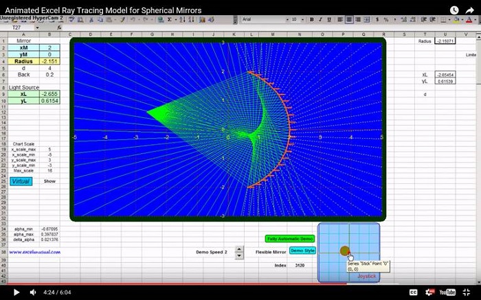
– We choose to have 21 rays emitted by the star and the rays will be uniformly covering the
mirror (there is a constant angle difference between two consecutive rays). The first and the
21st ray hit the edges of the mirror. The diagram above shows only 15 rays out a total of 21.
to be continued…
Hi George,
Your site is awesome! I just don’t have the right way to appreciate. I hope someday, you would like to consider putting this all in a nice book or booklets.
Specifically on optics, are you planning anytime to include things such as – lenses, prisms, microscopes, telescopes or more complex things? If not, where can one look at for information so that using your material on mirrors and this information, one can create material like you for these things?
regards,
Jagmohan
Thanks Jagmohan. I will do all those things. Telescopes have been my hobby for many years while in high school and college (at an experimental level). Right now I am trying to cover as much as possible in a short amount of time, so you need to be patient. What I have there will easily extend to lenses and group of components. I intend to do Maksutov, Schmidt, apochromat systems etc.
My stuff is done with more sweat than knowledge. You should try not to read too much but try to spend a lot of time building system models and knowledge. Outer information has a disastrous effect on creativity and motivation. Once the motivation is dead the mind is impotent. Spend a couple of months focusing 10-20 hours a week on it using Excel and the whole field will open to you, I guarantee. Persistance is everything. You can do better than I did, just be like a pitbull. Cheers, George
Bravo hombre! Saludos! That paragraph told me something more about yourself. I am touched.
Salut! I cannot stress this enough, you need a seed of knowledge but nowhere near the amount they try to force on you in school. The rest is a playful attitude (you have to do it for fun) and of course your own sweat. If you like to read and not take action (practice) books are good. Otherwise if you enjoy building stuff and experimenting, then most of reading goes against you. “Steal” ideas from books now and then but try to spend 99.9% of your time and energy practicing.
At the moment I would be hard pressed to explain something I do not fully understand. If I were to plot the time taken by a ‘test’ ray of light against the location within the lens through which the light passes what would I get? If the target were placed at the focal plane of the lens, the minimum would not be well defined. If I move back past the image, is the stationary path a minimum or is it now a local maximum?
To me is pretty clear now, choose anything other than the focal plane. Say a grid in front or after the focal plane. In the center you just get a ray along the optical axis. A very good place it to choose something right after the lens and then extend the rays after that in a straight line.
Very nice.
Here is an idea to consider: a spherical mirror gives a perfect image of a point situated at its center of curvature. That looks like a trivial case, but then start moving slowly away from the center, along the axis and across the axis. That will introduce mirror aberrations and give an intuitive feel for the nature of on-axis and off-axis imagery. It also shows that aberrations are dependent on conjugate location and will set you up for the discussion of other shapes, where the unaberrated point is at another location.
Fermat’s principle is a fundamental insight as Peter points out, but depends on how far you want to go with this.
Good luck with the site. Nice effort.
Thanks Dr. Mouroulis. Great to have you on the site! This will be a long therm effort. I am planning to do optics for few weeks this year but during several stretches. Now I will finish this (it will have incidence angle of the principal ray and the object distance as input parameters) an perhaps add an elliptical and a hyperboloidal mirror soon. Nest stretch will be some telescopes. Towards the end of the year I can do some of these: an achomat perhaps an apo and next year a Maksutow and a Schmidt. Actually next year I hope to get into more advanced aberration applications. Best regards, George
Thanks for the model, Peter. I opened it and it looks good. I will reply you in a while. It is good to start with raytracing first. The method you mention is apearently easier but when applied to a lens it might be a nightmare. Give me some time to ponder. I am just guessing yet.
I have got an initial demonstration of refraction at a convex lens working. In our earlier discussion you mentioned that you do not like the idea of using indirect tools, such as Solver, which add ‘one more veil on top of the issue’.
I would suggest that just because a cos(A) is easy to write and to construct on paper with ruler and compass it does not mean that the numerical analysis involved in its calculation is straightforward. min(T) is an equally well defined concept and very clear if you have the resources to produce a complete contour plot – you cannot get much more fundamental than an exhaustive search over options!
As for complexity, the use of Fermat’s principle does not require the use of angles calculated in 3d or other complex trigonometrical relationships. All it needs is a parametric representation of each surface and Pythagoras’s theorem for distance calculation. So far this appears to be working well; perhaps it would be possible to produce a complete virtual optical bench! Now that really is trying to run before walking/crawling are mastered.
Finally, why am I suggesting this could be investigated for your blog? The optics I remember from half a century ago was all about constructing diagrams with carefully drawn lines from the top of objects through the centers of idealised lenses and through their focal points – not too much insight. The direct use of stationary principles is both doable and, to the best of my limited knowledge, has novelty. Perhaps Dr Mouroulis might like to comment.
Peter, I need to look ito it and it certainly seems promissing. Could you please extend your example to a 25 ray model, on a convergent lens? I would like to benchmark it and get a feel of the speed. I will certainly finish what I started here but I am also willing to try the optimization path afterwards. It seems from what you say that there are a lot of possibilities with this tool and not only in optics. The carefully crafted diagrams certainly help with the understanding. I had a book (autor Tudor Bianu I believe) when I was in middle school with all those triangles and a million of notations and approximations. I tried in vain to understand it since I wanted to make a telescope. Now I can make anyting without any of that theory, just very basic principles and I think this is a good start. If the optimization is easier I am going to use it for sure later.
I will send you a workbook but it is all somewhat hand-crafted at the moment. A long way from the point where you can slide an optical element along a bench and see the image change! No promises as to whether that is even possible. I suspect that the right place for this in terms of your blog is ‘on the back burner’ waiting for a little more maturity.
Right now I appreciate anything with several rays just for comparison (25 would be ideal). I can wait.
Excel is a bitch. It gives me trouble with lines charted when one end is far away. The equation is correct, yet I get garbage on the chart. I wasted a lot of time and now I just create some special conditions (perhaps a custom function) to bring an artificial point closer to the edge of the chart. The model is practically done.
What do you mean a little maturity :-)?
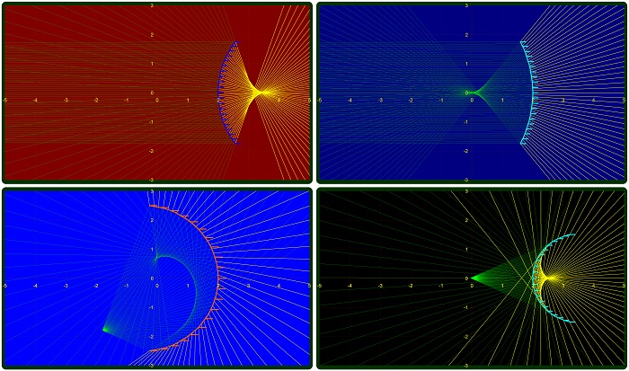
Lots of possibilities here. For example showing the cusp rather than clean focus for on axis reflection in spherical mirror; solved by parabolic mirror. Then there is ray tracing for diffraction.
Another aspect of ray tracing is to trace back from the observer to the source. That determines what you actually see. If you user the solver addin to Excel you could determine the path of a ray of light from the source to the observer by minimising the time of travel. Each point input to define an object would appear correctly placed on a ‘screen’ showing the ‘distorted’ image as seen.
Wouldn’t want you to settle for the easy options when I can produce ideas to really cause you grief 🙂
Peter, as opposed to the “ideal” approximations out there this model will show no clean focus.Things will be like in reality with the cusp. This will be a basic model so diffraction will be dealt with later and not in this series. The parabolic, elliptic and hyperbolic case will be dealt with soon, and of course comparisons must be shown. Since the spherical shape is the easiest to fabricate and by far the most common, I am starting with it. I am not sure I got your idea with tracing back the rays. In fact the sense of light travel is irrelevant in raytracing with no diffraction. I don’t use the solver since it’s a black box. It gives a sense of knowledge while spreading ignorance :-). Just like most of specialized black box packages out there.
I think the solver issue is where I disagree with you. It is fine to see you can work ideas up from first principles and do not have to rely on software packages you do not understand. At the same time the process should build an understanding of more complex concepts and it is the right thing to do to use the additional understanding as building blocks for further development.
To illustrate the concept that light always takes the quickest path it makes sense to calculate the time taken and minimise it. Complex manipulation of angles and equations, though representing a ‘first principles’ approach, will loose the message, not reinforce it.
By the way, the principle applies as much to reflection as it does to refraction. The sum of the time from the source to the mirror and from the mirror to the observer will be stationary with respect to changes of path.