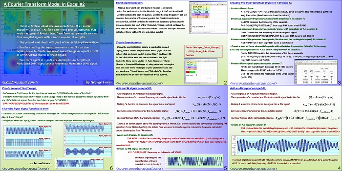
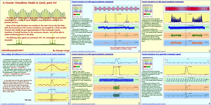
In this tutorial the Excel implementation of a Fourier transform is discussed. Seven input signals are created among which sinusoidal, rectangular and combinations of them.
A Dirac impulse, an amplitude modulated (AM) signal and a frequency modulated (FM) signal are also added among the input signal options.
![]()
A Fourier Transform Model in Excel #2
by George Lungu
– This is a tutorial about the implementation of a Fourier
transform in Excel. The first part went over adjustments that
make the general Fourier transform formula applicable on real
time sampled signals with a finite number of samples.
– This second part deals with part of the Excel implementation.
– Besides creating the input parameter area this section
explains how to create sinusoidal and rectangular inputs as well
as combinations (sums) of these signals.
– Two more types of inputs are developed, an Amplitude Modulated (AM) signal and a Frequency Modulated (FM) signal.
<excelunusual.com> by George Lungu
Excel implementation:
– Open a new workbook and name it Fourier_Tutorial.xls.
In the first worksheet enter the labels in range A1:A6 and in cell A11.
Cell B1 contains the start frequency, Cell B2 the stop frequency, cell B3
contains the number of frequency points the Fourier transform is
evaluated at, cell B4 contains the number of frequency points already
evaluated since the start of the “Calculate” macro, cell B5 contains the
time step for the input function and cell B11 contains the input function
selection (there will be 20 pre-selectable inputs).
Create three buttons:
– Using the control toolbox create a spin button named “Input_Select” and in the properties menu (right click the button while in design mode) change Min=1 and Max=20.
Private Sub Input_Select_Change()
[B11] = Input_Select.Value
End Sub
In the VBA editor write the macro shown to the right.
Make the Draw menu visible => Auto Shapes => Basic
Shapes = Rounded Rectangle => drag draw two rectangles.
Edit the color of the rectangle to your preference and add
text into them: “Reset” in one and “Calculate” in the other.
Two macros will be later associated to these buttons.
<excelunusual.com> 2
Creating five input functions (inputs # 1 through 5):
– Create a time column:
A41: “=0”, A421: “=A41+B$5” then copy cell A42 down to A5040. This will contain a 5000 cell
long time series (time increases down the column).
– Create an adjustable frequency sinusoid with amplitude 1 in column P:
Cell P38 contains the frequency of the sinusoid.
P41: “=SIN(2*PI()*P$38*$A41)” then copy P41 down to cell P5040.
– Create an adjustable frequency rectangular signal with amplitude of 1 in column Q:
Cell Q38 contains the frequency of the rectangular signal.
Q41: “=SIGN(SIN(2*PI()*Q$38*$A41))” then copy Q41 down to cell Q5040.
– Create a sum of the previous two signals (the sine and the rectangular signal) in column R:
R41: “=P41+Q41” then copy R41 down to cell R5040.
– Create a sum of three sinusoidal signals with adjustable frequencies (situated in the range
S36:S38) and amplitudes of: 1, 0.5 and 0.3 respectively, in column S:
Range S36:S38 contains the frequencies of the three sinusoids.
S41: “=SIN(2*PI()*S$38*$A41)+0.5*SIN(2*PI()*S$37*$A41)+0.3*SIN(2*PI()*S$36*$A41)” then
copy S41 down to cell S5040.
– Create a Dirac signal approximation in column T:
Firstly, set everything in the range T41:T4040 to zero.
Then change cell’s T2540 value to: “=T38”.
Cell T38 will contain the magnitude of the Dirac signal
(set to 100).
<excelunusual.com> 3
Add an AM signal as input #6:
– An AM signal is an Amplitude Modulated signal.
– The expression of a constant amplitude sinusoidal signal looks like this: x(t) Asin( 2f t )
– Making A a function of time turns the signal into a AM signal:
x (t) A(t)sin( 2 f t )
AM
– Let’s use a slower sinusoid as the modulation signal: A(t) 10.5sin( 2 f t )
modulation
– The final formula of the AM signal becomes: x (t) 10.5sin( 2 f t)sin( 2 f t )
AM modulating carrier
– Create an AM signal in column U:
Cell U34 contains the modulating frequency and U37 contains the modulated (or carrier) frequency.
U41: “= (1+0.5*SIN(2*PI()*U$34*$A42))*SIN(2*PI()*U$37*$A42)” then copy U41 down to cell U5040.
0 20 40 60 80 100
The result of plotting range U41:U5040 function of time (range A41:A5040) on a scatter chart, for a carrier frequency
of 0.7 Hz and a modulating frequency of 0.05 Hz is seen in the above chart.
<excelunusual.com> 4
Add an FM signal as input #7:
– An FM signal is an Amplitude Modulated signal.
– The expression of a constant frequency sinusoidal signal looks like this: x(t) sin( 2f t )
– Making f a function of time turns the signal into a AM signal:
x (t) sin( 2 f (t )t )
FM
– Let’s use a slower sinusoid as the modulation signal: f (t) f 0.3sin( 2f t )
carrier modulation
– The final formula of the FM signal becomes: x (t) sin(2f 0.3sin( 2 f t)t )
FM carrier modulation
– There is an earlier tutorial about FM signals posted in March 2011 which explains the correct way of creating FM
signals in Excel. Without getting into details here we need to insert a special column for the phase calculation
before obtaining the final FM column.
-Create an FM phase in column AK:
Cell AK34 contains the modulating frequency and AK38 contains the modulated (carrier) frequency.
AK41: “=0”, AK42: “=AK41+2*PI()*(AK$34+0.3*SIN(2*PI()*AK$38*A42))*B$5” then copy AK42 down
to cell AK5040.
– Create an FM signal in column V:
V41: “=SIN(AK41)” then copy V41 down to cell V5040.
The result of plotting the FM signal function of time is seen in the chart to the right:
<excelunusual.com> 5
Create an input “hub” range:
– Let’s create a “hub” range for the input signal, and use B41:B5040 as location of this “hub”
– Using the numerical value in the “Input_Select” range (cellB1) this hub will selectively collect input data from
any of the 20 input signals from the input data range ( P41:AI5040 ).
– B41: “=OFFSET(P41,0,B$11-1)” then copy B41 down to cell B5040.
Chart the input signal function of time:
– Create a 2D scatter chart having x-values in the range A41:A5040 and y-values in the range B41:B5040 and
label it “Input_Signal”.
– Verify that when the “Input_Select” value is changed the chart displays a different input signal.
2
1.5 Input_Signal = 4
1.5 1
Input_Signal = 1 0.5
100 Input_Signal = 5
1.5 80
Input_Signal = 2
0 0 20 40 60 80 100 120
1.5 Input_Signal = 6
3 1
Input_Signal = 3 0.5
Input_Signal = 7
to be continued… 0 0 20 40 60 80 100 120
by George Lungu <excelunusual.com> 6


EXCELlent