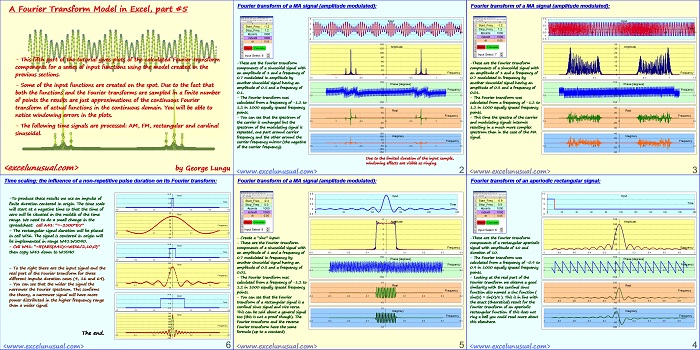
This part of the tutorial demonstrates the Fourier transform operation in a few cases of periodic and non-periodic signals, such as an AM signal, an FM signal, a rectangular non repetitive signal and a cardinal sine signal.
The last slide contains an application to the scaling property of the Fourier transform on a non-repetitive time signal. It actually shows that spreading a signal in the time domain shrinks its spectrum and vice versa.
![]()
A Fourier Transform Model in Excel, part #5
by George Lungu
– This fifth part of the tutorial gives plots of the calculated Fourier transform
components for a series of input functions using the model created in the
previous sections.
– Some of the input functions are created on the spot. Due to the fact that
both the functions and the Fourier transforms are sampled in a finite number
of points the results are just approximations of the continuous Fourier
transform of actual functions in the continuous domain. You will be able to
notice windowing errors in the plots.
– The following time signals are processed: AM, FM, rectangular and cardinal
sinusoidal.
<excelunusual.com> by George Lungu
Fourier transform of a MA signal (amplitude modulated):
-These are the Fourier transform components of a sinusoidal signal with an amplitude of 1 and a frequency of Frequency modulated in amplitude by
another sinusoidal signal having an amplitude of 0.5 and a frequency of 50
– The Fourier transform was calculated from a frequency of -1.2 to -150
in 1000 equally spaced frequency 100
– You can see that the spectrum of 0
the carrier is unchanged but the -50
spectrum of the modulating signal is
-repeated, one part around carrier
frequency and the other around the 100 Imaginary carrier frequency mirror (the negative of the carrier frequency).
Due to the limited duration of the input sample,
windowing effects are visible as ringing.
Fourier transform of a FM signal (frequency modulated):
-These are the Fourier transform components of a sinusoidal signal with
an amplitude of 1 and a frequency of Frequency modulated in frequency by
another sinusoidal signal having an amplitude of 0.3 and a frequency of 0.01.
-1.5 -1 -0.5 -50 0 0.5 1 1.5
– The Fourier transform was
calculated from a frequency of -1.2 to -150
in 1000 equally spaced frequency 40
points.
– This time the spectra of the carrier and modulating signals intermix -20
resulting in a much more complex spectrum than in the case of the MA signal.
20
Frequency
0
-1.5 -1 -0.5 0 0.5 1 1.5
-20
-40
Fourier transform of an aperiodic rectangular signal:
-These are the Fourier transform
components of a rectangular aperiodic
signal with amplitude of 10 and duration of 10. -1
-0.8 -0.6 -0.4 -0.2 0 0.2 0.4 0.6 0.8 1
– The Fourier transform was calculated from a frequency of -0.9 to 0.9 in 1000 equally spaced frequency points.
-1 -0.8 -0.6 -0.4 -0.2 -50 0 0.2 0.4 0.6 0.8 1
– Looking at the real part of the
Fourier transform we observe a good similarity with the cardinal sinus 100
function also named a sinc function ( 50
sinc(x) = sin(x)/x ). This is in line with
the exact (theoretical) result for the
Fourier transform of an non-periodic rectangular function. If this does not ring a bell you could read more about this elsewhere.
Fourier transform of a MA signal (amplitude modulated):
– Create a “sinc” input:
– These are the Fourier transform components of a sinusoidal signal with an amplitude of 1 and a frequency of -0.4 -0.3 -0.2 -0.1 0 0.1 0.2 0.3 0.4
0.7 modulated in frequency by another sinusoidal signal having an amplitude of 0.3 and a frequency of 0.01.
– The Fourier transform was calculated from a frequency of -1.2 to 10 in 1000 equally spaced frequency points. 0
-0.4 -0.3 -0.2 -0.1 0 0.1 0.2 0.3 0.4
– You can see that the Fourier transform of a rectangular signal is a cardinal sinus signal and vice versa.
This can be said about a general signal too (this is not a proof though). The Fourier transform and the reverse Fourier transform have the same formula (up to a constant)
Time scaling: the influence of a non-repetitive pulse duration on its Fourier transform:
-To produce these results we use an impulse of finite duration centered in origin. The time scale will start at a negative time so that the time of -150 -100 -50 0 50 100 150
zero will be situated in the middle of the time range.
We need to do a small change in the spreadsheet: cell A41: “=-2500*B5”
– The rectangular signal duration will be placed in cell W36. The signal is centered in origin will be implemented in range W41:W5040.
– Cell W41: “=IF(ABS(A41)<=W$36/2,10,0)”
then copy W41 down to W5040 4.8 Time
-150 -100 -50 0 50 100 150
– To the right there are the input signal and the real part of the Fourier transform for three different impulse duration cases (4, 16 and 64).
0
– You can see that the wider the signal the narrower the Fourier spectrum. This confirms
the theory, a narrower signal will have more Input power distributed in the higher frequency range than a wider signal.
-150 -100 -50 0 50 100 150
by George Lungu <excelunusual.com>


Fantastic works ! Thank you Sir !
Hi George, I did create a sinus function with amplitude of 20 and frequency of 200Hz then I used the built-in FFT function in Excel the results I have got were different than what I expect, i.e, amplitude of 18 instead of 20, and the frequency 29Hz rather than 200Hz, I couldn’t figure it out why. I did use your template for the same function, the amplitude was 0.6 and the frequency 29. So both calculation gave different answers. Shall I send you the files? you may have the answer for that ? PS: my knowledge in this area are very limited. By the way your template is it DFT or FFT ?
Great work keep it up! I’m currently working on examining accelerometer data from walk trips and thinking of using this technique to count steps. Do you think that is an effective technique for that purpose? I would use the amplitude values above certain threshold levels to identify step counts.
Yes, you definitely need to try. I am a little sceptical about applying the FT at counting steps but it would be interesting to experiment it on the data. Take data and put it in excel. Also do both integration and derivation on the original data and run different tests on all these stacks of data. These are just some wild guesses. You need to practically experiment with this yourself. Also if you have more time you could look into Kalman filters but also try various simple filters (low pass, high pass, band pass, FIR, IIR). All of there are easy and fun to implement in Excel. Your original idea with a simple threshold might work satisfactorily though. Play with a basic moving average filter before thresholding to get rid of noise. Good luck, George
Hi George, Sorry I can’t see the email address!
Tarek, go to the “About” page on the top menu. There is a “Contact me at:” on that page.
Hi George,
Thank you for your reply. Just to give you an idea about the problem that I am facing. I have 8m /s airflow of over a hard disk and I am looking to find out if the airflow is inducing the vibration of the disk. I did a transient computational fluid dynamics (CFD) simulation of the air flow over the disk, as results I have the pressure as function of time. I have been advised to record the pressure on different points and use the FFT to calculate the amplitude vs frequency, the sound level pressure (SPL) vs frequency. At this stage I will focus on analysing the data recorded on points before moving to surfaces. The outcome of the FFT calculation based on CFD analysis will be then compared to Finite Element Analysis (FEA). If the amplitudes are intersecting at the same frequencies, then that would answer my question about the cause of the disk vibration.
Example of the data:
time [s] Point 1 (Pressure) [Pa] Point 2 (Pressure) [Pa] Point 3 (Pressure) [Pa]
0.00001 2.78E-04 4.61E-04 1.21E-05
0.00002 1.45E-01 2.91E-02 -5.91E-04
0.00003 -2.05E-02 2.99E-02 -3.65E-03
0.00004 3.05E-01 3.79E-02 -9.40E-03
0.00005 -5.18E-02 -1.02E-02 -1.61E-02
0.00006 9.85E-01 1.15E-01 -9.77E-03
0.00007 3.41E+00 5.79E-01 -1.57E-02
I have 38000 sampling data. I can send you the data if want.
I really appreciate your help.
Tarek
Tarek, firstly this site is for fun and inspiration only. Please don’t take anything from here to be used to design something that might put people’s life at risk. I am an electrical engineer and I do all of these things for fun myself since the life out there in industry can be quite boring. Within the next couple of years I will get to very advanced stuff here, and CFD and FEA will be prime subjects. I can help you with the FT. FFT and DFT (discrete) do the same thing just FFT saves some time. In your case you don’t mind if the computation takes 2 seconds or 5 seconds to plot a chart so just use DFT. To begin with, my worksheet is good enough, you just need to extend the number of time points to accommodate 38000. Sure, send me the file (in the About there is an email address) but keep working on it yourself too. Let’s keep the communication on the comment section – HERE. I need comments. Cheers, George
Hi,
Thank you for the spreadsheet. I would like to ask you question. I have pressure times histories over a surface. I would like to calculate the SPL and the amplitudes by using the FFT. Could you please show me how to do it. Thank you in advance. Tarek
Tarek, due to my busy schedule I don’t promise anything but I will try. Please define your problem. Is a 3D surface? What is SPL? Do you have a function of pressure function of time (history)? George