Spectral Analysis – a Fourier transform tutorial – part #1

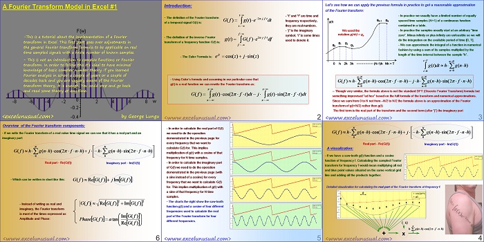
This is a basic tutorial about implementation of a standard Fourier transform model in Excel. It is not an introduction to Fourier analysis.

You could choose to familiarize yourself with the subject before proceeding with this tutorial. Solving a few Fourier transform excersises would be of help too.

Essentially, this part shows you how to adapt the general Fourier formula for a continuous real signal to a sampled signal having a limited number of samples.

A Fourier Transform Model in Excel #1

by George Lungu

-This is a tutorial about the implementation of a Fourier
transform in Excel. This first part goes over adjustments in
the general Fourier transform formula to be applicable on real
time sampled signals with a finite number of known samples.

– This is not an introduction to complex functions or Fourier
transform. In order to follow this it’s ideal to have minimal
knowledge of basic complex number theory.

If you learned Fourier analysis in school a couple of years or a couple of
decades back and you are vaguely aware of the Fourier
transform theory, it is enough.

You could stop and go back and read some theory at any time.

<excelunusual.com> by George Lungu

Introduction:

– “t” and “f” are time and
– The definition of the Fourier transform
G(f )  g(t)e dt frequency respectively,
of a temporal signal G(t) is:
they are real numbers.
– “j” is the imaginary
f
symbol, “i” is some times
– The definition of the inverse Fourier 2jf t
g(t) G(f )e df used to denote it.

transform of a frequency function G(f) is:
f
jz
– The Euler Formula is: ecos(z) jsin(z )
– Using Euler’s formula and assuming in our particular case that
g(t) is a real function we can rewrite the Fourier transform as:

G( f )  g(t)  cos(2 f  t)dt j  g(t) sin( 2 f  t)dt

<excelunusual.com> 2

Let’s see how we can apply the previous formula in practice to get a reasonable approximation of the Fourier transform:

– In practice we usually have a limited number of equally spaced time samples of a continuous function contained in a table.
gN-1 gN  (N+1)
g(t)

We used the – In practice the samples usually start at an arbitrary “time zero”. Minus infinity or plus infinity are unfeasible so we will
do the integration on the available period of time [0, T].

– We can approximate the integral of a function in numerical
fashion by using a sum of its samples multiplied by the
length of the time interval between the sample “h”.

– Though very similar, the formula above is not the standard DFT (Discrete Fourier Transform) formula but
something improvised “ad hoc” based on the full formula of the transform and numerical approximations.

Since we sum from 0 to N not from -N/2 to N/2 the formula above is an approximation of the Fourier
transform of g(t+N/2) rather then g(t)

The first term is the real part of the transform and the second term (after “j”) the imaginary part

<excelunusual.com> 3

Real part – Re(G(f)) Imaginary part – Im(G(f))

A visualization:

3.5
– If we have a saw-tooth g(t) function and a cosine function of frequency f. Calculating the sampled Fourier transform for frequency f would mean multiplying all red and blue point values situated on the same vertical grid line and adding all the products together.

Detailed visualization for calculating the real part of the Fourier transform at frequency f:

3 h cos(2pi*f*t)
2.5 g(t)

RFT – Redneck Fourier Transform
<excelunusual.com> 4

3.5
cos(2pi*f*t)

– In order to calculate the real part of G(f) we need to do the operation demonstrated in the previous page for every frequency that we want to calculate G(f) for. This implies
multiplication of g(t) with a cosine of that g(t) frequency for N time samples.

– In order to calculate the imaginary part of G(f) we need to do the operation demonstrated in the previous page (with a sine instead of a cosine) for every frequency that we want to calculate G(f)
for. This implies multiplication of g(t) with a sine of that frequency for N time samples.

– The charts the right show the saw-tooth function g(t) and a cosine of four different g(t) frequencies used to calculate the real part of the Fourier transform for four different frequencies.

<excelunusual.com> 5

Overview of the Fourier transform components:

– If we write the Fourier transform of a real value time signal we can see that it has a real part and an
imaginary part:

Real part – Re(G(f)) Imaginary part – Im(G(f))

– Which can be written in short like this:
G( f )  Re G (f ) jIm G (f)

– Instead of writing as real and G( f )  Re  G( f )   Im  G (f )  imaginary, the Fourier transform is most of the times expressed as
 Im  G( f )  
Amplitude and Phase:
Phase  G( f )   atan

Re  G( f ) 

by George Lungu <excelunusual.com> 6