TRANSPOSE() & MMULT() – two important Excel spreadsheet functions for matrix manipulations

This is a tutorial introducing two important matrix manipulation spreadsheet functions in Excel: the matrix transposition function TRANSPOSE() and the matrix multiplication function MMULT().

These functions are a bit harder to use than the regular spreadsheet functions in the sense that the result is a matrix and a matrix cell range is treated by the program as a unity (you cannot change the formula since you cannot operate on a single cell).

There are some basic rules to follow while entering or modifying such arrays.  A bench-marking post will follow in which the two matrix functions will be compared speed wise with regular spreadsheet functions and also with user defined custom VBA functions.

[sociallocker][/sociallocker]

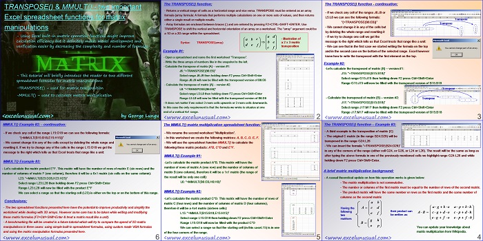
TRANSPOSE() & MMULT() – two important Excel spreadsheet functions for matrix manipulations

by George Lungu

– Using Excel built-in matrix operation functions might improve
calculation efficiency but it definitely makes model development and
verification easier by decreasing the complexity and number of formulas.

– This tutorial will briefly introduce the reader to two different
spreadsheet formulas for matrix manipulations:

-TRANSPOSE() – used for matrix transposition

-MMULT() – used to calculate matrix multiplication

<excelunusual.com> by George Lungu

The TRANSPOSE() function:

– Returns a vertical range of cells as a horizontal range and vice versa. TRANSPOSE must be entered as an array
formula (array formula: A formula that performs multiple calculations on one or more sets of values, and then returns
either a single result or multiple results.

– Array formulas are enclosed between braces { } and are entered by pressing F2+CTRL+SHIFT+ENTER. Use
TRANSPOSE to shift the vertical and horizontal orientation of an array on a worksheet. The “array” argument could be
a 1D or a 2D range within the spreadsheet.

Syntax: TRANSPOSE(array)  b e
a 2 x 3 matrix
d e f
transposition
c f

Example #1:

– Open a spreadsheet and name the first worksheet “Transpose”.

– Write the three arrays of numbers like in the snapshot to the left.

– Calculate the transpose of matrix {A} – version #1:
J6: “=TRANSPOSE(B6:E6)”
Select range J6:J9 then holding down F2 press Ctrl+Shift+Enter
Range J6:J9 will now be filled with the transposed version of B6:E6

– Calculate the transpose of matrix {A} – version #2:
L8: “=TRANSPOSE(B6:E6)”
Select range L5:L8 then holding down F2 press Ctrl+Shift+Enter
Range L5:L8 will now be filled with the transposed version of B6:E6

– It does not matter if we select 3 more cells upwards or 3 more cells downwards.
In this case the only requirement is that the formula we wrote is situates at one
end of a vertical 4×1 range.

<excelunusual.com> 2

The TRANSPOSE() function – continuation:

– If we check any cell of the ranges J6:J9 or
L5:L8 we can see the following formula:
Transpose
“{=TRANSPOSE(B6:E6)}”
Transpose

– We cannot change it in any of the cells but
by deleting the whole range and rewriting it

– If we try to change one cell we get the
message to the right which tells us that Excel treats that range like a unity:

– We can see that in the first case we started writing the formula on the top
and in the second case on the bottom of the selected range. Excel however
knew how to write the transposed with the first element on the top.

Example #2:

-Let’s calculate the transposed of matrix {B} – version #1:

J15: “=TRANSPOSE(B15:B18)”
Select range G15:J15 then holding down F2 press Ctrl+Shift+Enter
Range G15:J15 will now be filled with the transposed version of B15:B18
Transpose

– Calculate the transposed of matrix {B} – version #2:
Transpose

J17: “=TRANSPOSE(B15:B18)”
Select range J17:M17 then holding down F2 press Ctrl+Shift+Enter
Range J17:M17 will now be filled with the transposed version of B15:B18
<excelunusual.com> 3

The TRANSPOSE() function – Example #3:

– A third example is the transposition of matrix {C}

– The original C matrix (in the range B24:D29) will be
transposed in the range G24:L26

– We can insert the formula “=TRANSPOSE(B24:D29)”
in any of the corners of the range (either cell G24, or G26, or L24 or L26). The result will be the same as long as
after typing the above formula in one of the previously mentioned cells we highlight range G24:L26 and while
holding down F2 press Ctrl+Shift+Enter.

A brief matrix multiplication background:

– A casual theoretical update on how this operation works is given below:

– The matrix multiplication is not commutative.

– The number or columns of the first matrix must be equal to the number of rows of the second matrix.

– The product matrix will have the same number or rows as the first matrix and the same number of
columns as the second matrix

You can update your knowledge about
matrix multiplication from Wikipedia.

<excelunusual.com> 4

 

The MMULT() matrix multiplication spreadsheet function:

– We rename the second worksheet “Multiplication”.

– In this worksheet we create the following matrices: A, B, C, D, E, F.

– We will use the spreadsheet function MMULT() to calculate the
following three matrix products: A*B, C*D and E*F.
MMULT() Example #1:

-Let’s calculate the matrix product A*B. This matrix will have the
number of rows of matrix A (one row) and the number of columns of
matrix B (one column), therefore it will be a 1×1 matrix (the range of
the result will be only one cell):
L6: “=MMULT(B6:E6,H6:H9)”
MMULT() Example #2:

-Let’s calculate the matrix product C*D. This matrix will have the number of rows of
matrix C (four rows) and the number of columns of matrix D (four columns),
therefore it will be a 4×4 matrix (sixteen cells):

L15: “=MMULT(B15:B18,E15:H15)”
Select range L15:O18 then holding down F2 press Ctrl+Shift+Enter
Range L15:O18 will now be filled with the product C*D
We can select a range so that the starting cell (in this caseL15) is in one
of the four corners of the range.

<excelunusual.com> 5

MMULT() Example #2: – continuation:

– If we check any cell of the range L15:O18 we can see the following formula:
“{=MMULT(B15:B18,E15:H15)}”

– We cannot change it in any of the cells except by deleting the whole range and
rewriting it. If we try to change any of the cells in the range L15:O18 we get the
message to the right which tells us that Excel treats that range like a unity:
MMULT() Example #3:

– Let’s calculate the matrix product E*F. This matrix will have the number of rows of matrix E (six rows) and the
number of columns of matrix F (one column), therefore it will be a 6×1 matrix (six cells on the same column):
L23: “=MMULT(B23:D28,H23:H25)”
Select range L23:L28 then holding down F2 press Ctrl+Shift+Enter
Range L23:L28 will now be filled with the product E*F
We can select a range so that the starting cell (L23) is either on the top or on the bottom of this range.

Conclusions:

– The two spreadsheet functions presented here have the potential to improve productivity and simplify the
worksheet while dealing with 2D arrays. However some care has to be taken while writing and modifying
these matrix formulas (F2+Ctrl+Shift+Enter & treat a matrix result like a unity).

– A bench-marking file will be created in a future tutorial which will try to compare the speed of 2D matrix
manipulations in three cases: using simple built-in spreadsheet formulas, using custom made VBA formulas
and using the matrix manipulation formulas presented here.

by George Lungu <excelunusual.com> 6