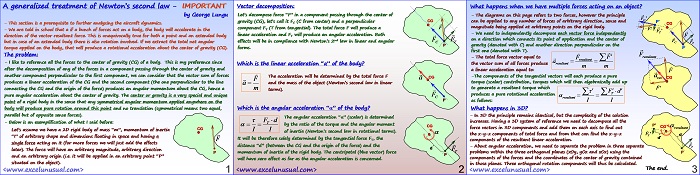
Most of people have heard of Newton’s second law, mass, moment of inertia or the definition of the acceleration both linear and angular. The stuff presented here is elementary (9th grade), yet it is generally not properly understood. What happens when one applies a bunch arbitrary forces on an arbirtarily shaped body? The resultant force vector produces a linear acceleration… Read More... "Newton Generalized Treatment"
This category hosts engineering animated models in MS Excel. Excel is particularly valuable in engineering being inexpensive and ubiquitous. In my career I managed to solve difficult engineering problems by building animated simulations where engineers using other, much more expensive software, failed. Unlike dedicated engineering software, excel is not a “black box”, which means that you develop your models from scratch using basic principles, calculations and charting. This leads to a much better understanding and control of the problem.
Excel is a great software for engineering calculations because it can combine data tables, charts and even engineering formulas under the same application.As far as civil engineering is concerned, Excel can do regular calculations such as cost estimates, schedule and cost control, and markup estimation, as well as structural calculations of reactions, stresses, strains, deflections, and slopes. Excel can deal with difficult problems, charting, and report generation.
Longitudinal Aircraft Dynamics #4 – virtual aircraft definition
This section of the tutorial explains how to create the 2D aircraft components for the animated longitudinal stability model. The first part deals with extracting the x-y coordinates for the fuselage, canopy, vertical stabilizer and rudder. The second part handles the main wing airfoil and the horizontal stabilizer airfoil. All thses parts will be put together in the next section.… Read More... "Longitudinal Aircraft Dynamics #4 – virtual aircraft definition"
Longitudinal Aircraft Dynamics #3 – layout parameters and wireframe fuselage generation
This section discusses the layout of the virtual plane and provides for the worksheet implementation of the plane dimensions as input parameters controlled by spin buttons and macros. In the final part a freeform is used to generate raw data for the fuselage. [sociallocker][/sociallocker] Longitudinal Aircraft Dynamics #3- defining the virtual aircraft by George Lungu – This section of the tutorial… Read More... "Longitudinal Aircraft Dynamics #3 – layout parameters and wireframe fuselage generation"
Longitudinal Aircraft Dynamics #2 – 2D polynomial interpolation of parameters cl, cd and cm
In the previous section, the main wing airfoil and the horizontal stabilizer airfoil were simulated using Xflr5. The three coefficients, lift, drag and moment were then interpolated on charts in Excel using 4th and 5th order polynomials. This section shows a few tricks about how to easily introduce those 60 equations as spreadsheet formulas in Excel ranges. It also presents a simple linear interpolation method across the Reynolds… Read More... "Longitudinal Aircraft Dynamics #2 – 2D polynomial interpolation of parameters cl, cd and cm"
Longitudinal Aircraft Dynamics #1 – using Xflr5 to model the main wing, the horizontal stabilizer and extracting the polynomial trendlines for cl, cd and cm
This is a tutorial about using a free aerodynamic modeling package (Xflr5) to simulate two airfoils in 2D (the main wing and the horizontal stabilizer) for ten different Reynolds numbers, then using Excel to extract the approximate polynomial equations of those curves (cl, cd and cm) and based on them, simulate a 2D aircraft as an animated model. This section deals with… Read More... "Longitudinal Aircraft Dynamics #1 – using Xflr5 to model the main wing, the horizontal stabilizer and extracting the polynomial trendlines for cl, cd and cm"
Aerodynamics Naive #3 – a brief introduction to Xflr5, a virtual wind tunnel
The previous section implemented and charted the ping-pong polar diagrams in a spreadsheet and showed a reasonable similarity, for moderate angles of attack, between these diagrams and the ones modeled using Xflr5, a virtual wind tunnel. This section introduce the concept Reynolds number and it also contains a very brief introduction to Xflr5, the free virtual wind tunnel software. Aerodynamics… Read More... "Aerodynamics Naive #3 – a brief introduction to Xflr5, a virtual wind tunnel"
Aerodynamics Naive #2 – spreadsheet implementation of the Ping-Pong polar diagrams
This section of the tutorial implements the lift and drag formulas in a worksheet, creating and charting the polar diagrams for an ultra simplified ping-pong model of an airfoil. Comparing these diagrams with ones obtained by using a virtual wind tunnel (XFLR5) we can see a decent resemblance for moderate angles of attack (smaller than about 8 degrees in absolute value).… Read More... "Aerodynamics Naive #2 – spreadsheet implementation of the Ping-Pong polar diagrams"
Aerodynamics Naive #1 – deriving the Ping-Pong airfoil polar diagrams
This is the ping-pong aerodynamic analogy. The wing is a ping pong bat and the air is a bunch of evenly spaced array of ping pong balls. It is a naive model but, as we will see in a later post, the polar diagrams derived from this analogy (between -12 to +12 degrees of angle of attack) are surprisingly close shape wise to the real diagrams of a thin,… Read More... "Aerodynamics Naive #1 – deriving the Ping-Pong airfoil polar diagrams"
How Do They Fly? – an intuitive look into lift generation and flight stability
Have you ever wondered why the flight attendants of a half empty airliner talk people into moving to the front half of the plane? Have you ever wondered why a flying wing can fly without a tail or why the stability of some of these flying wing can be controlled only by computer? Or why a 12 pack stored in at… Read More... "How Do They Fly? – an intuitive look into lift generation and flight stability"
A 2D Demo for Spherical Mirrors in Excel – with virtual reflected rays
This is a demonstrative model for 2D spherical mirror ray tracing in Excel displaying both the real reflected rays and the virtual reflected rays. You you have the option of turning the visibility of the virtual rays off if you wish. It works in Excel 2003 at about 40 frames per second and in Excel 2007 at about 4 frames per second.… Read More... "A 2D Demo for Spherical Mirrors in Excel – with virtual reflected rays"
Introduction to Geometrical Optics – a 2D ray tracing Excel model for spherical mirrors – Part 7
Based on the formulas derived up to this point in the series, this section creates an improved custom VBA function which calculates the x-y Cartesian coordinates of three points: the incident point, the terminal point of the real reflected ray and the terminal point of the virtual reflected ray. The structure of the function is fairly simple and it is… Read More... "Introduction to Geometrical Optics – a 2D ray tracing Excel model for spherical mirrors – Part 7"
Introduction to Geometrical Optics – a 2D ray tracing Excel model for spherical mirrors – Part 6
This section simplifies the formula for the Cartesian coordinates of the terminal point of the reflected ray and derives a very similar formula for a terminal point of the virtual reflected ray. In the next section all these new formulas together with some old formulas will be combined into a new user defined VBA function which will be used alone… Read More... "Introduction to Geometrical Optics – a 2D ray tracing Excel model for spherical mirrors – Part 6"
Introduction to Geometrical Optics – a 2D ray tracing Excel model for spherical mirrors – Part 5
This brief section takes the two previously created custom VBA functions (Reflect() and Chart_Reflect()) and use them to create the data for both the incident and the reflected bundles of rays within the same table. The data is then plotted on the same chart with the mirror and the result is a preliminary model which you can experiment with. [sociallocker][/sociallocker]… Read More... "Introduction to Geometrical Optics – a 2D ray tracing Excel model for spherical mirrors – Part 5"
A Preliminary 2D Ray Tracing Demo for Spherical Mirrors in Excel
This is a demonstrative model for 2D spherical mirror ray tracing in Excel. It works in Excel 2003 at about 40 frames per second and in Excel 2007 at about 4 frames per second. You can start it in a hands-off demo mode by clicking the “Fully Automatic Demo” button and at any time you can hit the the “Demo… Read More... "A Preliminary 2D Ray Tracing Demo for Spherical Mirrors in Excel"